
ENCM-100 · Lesson 5 of 5 · 34 min
Lists, files and numerical work
Engineering data comes in quantity: a load test with hundreds of readings, a year of hourly flows, the coordinates of every node in a truss. This final chapter gives you the tools to hold, read, process and plot that data. It covers Python's lists and dictionaries, reading and writing files, and then the NumPy library, which turns Python into a serious numerical tool. The examples bring together the course and much of first year: fitting a line to test data to find Young's modulus, integrating flow measurements, solving the three-cable system from Statics with one line of code, and simulating cooling with Euler's method.
Lists
A list is an ordered collection of values in square brackets. Lists can hold any type, can grow and shrink, and are the everyday container for a series of readings.
strain = [612, 655, 701, 748, 790, 823, 845, 812, 776, 731]
print(len(strain), strain[0], strain[-1])
print(strain[2:5], strain[:3])
strain.append(702)
print(len(strain), sum(strain) / len(strain))
print(min(strain), max(strain), sorted(strain)[:3])
10 612 731
[701, 748, 790] [612, 655, 701]
11 745.0
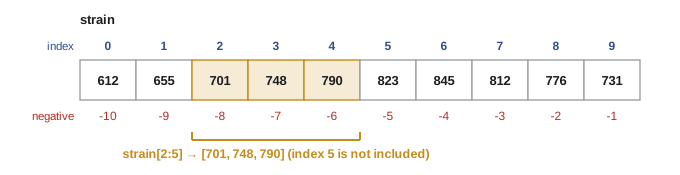
612 845 [612, 655, 701]Indexing starts at 0, so strain[0] is the first item and strain[9] the tenth; negative indexes count from the end, so strain[-1] is the last. A slice a[start:stop] takes items from start up to but not including stop, the same convention as range(). Methods change a list in place: append() adds an item, insert() puts one at a position, remove() deletes the first matching value, and sort() sorts the list itself (sorted() returns a sorted copy and leaves the original alone).
List comprehensions
A list comprehension builds a new list by applying an expression to each item of another, optionally with a condition. It replaces a common three-line loop with one readable line.
pressures_psi = [100, 150, 250]
pressures_kPa = [round(p * 6.894757, 1) for p in pressures_psi]
print(pressures_kPa)

strain = [612, 655, 701, 748, 790, 823, 845, 812, 776, 731]
high = [s for s in strain if s > 800]
print(high)
Output: [689.5, 1034.2, 1723.7] and [823, 845, 812].
Dictionaries
A dictionary maps keys to values, like a lookup table. It is ideal for material properties, section tables, or any data where you look things up by name rather than by position.
E_MPa = {"steel": 200000, "aluminium": 69000, "timber": 11000}

material = "aluminium"
print(f"E for {material}: {E_MPa[material]} MPa")

E_MPa["concrete"] = 25000            # add an entry
for name, E in E_MPa.items():
    print(f"{name:<10}{E:>8}")
Looking up a key that is not there raises a KeyError; E_MPa.get("glass") returns None instead, and "glass" in E_MPa tests whether the key exists. (The moduli here are typical textbook values; real design uses the values specified in the governing standard for the particular grade.)
Reading and writing files
Data usually arrives in files, most often CSV (comma-separated values), which every spreadsheet, data logger and database can produce. Python's with open(...) statement opens a file and guarantees it is closed afterwards, and the csv module handles splitting lines into fields correctly.
Worked problem
A tensile test file
Write a small CSV file of load-extension readings from a tensile test, then read it back into two lists of numbers.
Show solution
import csv # Write the file (normally the test machine produces this) rows = [(0, 0.000), (5, 0.045), (10, 0.087), (15, 0.134), (20, 0.176), (25, 0.222), (30, 0.264)] with open("tensile.csv", "w", newline="") as f: writer = csv.writer(f) writer.writerow(["load_kN", "extension_mm"]) writer.writerows(rows) # Read it back load, ext = [], [] with open("tensile.csv", newline="") as f: reader = csv.reader(f) next(reader) # skip the header row for row in reader: load.append(float(row[0])) ext.append(float(row[1])) print(load) print(ext)- Output: [0.0, 5.0, 10.0, 15.0, 20.0, 25.0, 30.0] and [0.0, 0.045, 0.087, 0.134, 0.176, 0.222, 0.264].
Answer: Values read from a file are strings, so each is converted with float(). Skipping the header with next(reader) is a frequent need; forgetting it gives a ValueError when Python tries to convert "load_kN" to a number
Files are where real-world data is messiest: missing values, extra spaces, units in the header, a summary line at the bottom. Always look at a few lines of a new data file before writing code to read it, and check the number of rows read against what you expect.
NumPy: arrays and vectorized calculation
NumPy is the foundation of scientific Python. Its array type holds numbers of one type in a compact block of memory, and arithmetic on an array applies to every element at once, without writing a loop. This vectorized style is shorter, closer to the mathematics, and typically tens to hundreds of times faster than a Python loop for large data.
import numpy as np

strain = np.array([612, 655, 701, 748, 790, 823, 845, 812, 776, 731])
stress_MPa = 200000 * strain * 1e-6      # E times strain, every element at once
print(stress_MPa)
print(strain.mean(), strain.max(), np.std(strain, ddof=1))
print(strain[strain > 800])              # boolean selection

x = np.linspace(0, 6, 4)                 # 4 evenly spaced points from 0 to 6
print(x)
[122.4 131. 140.2 149.6 158. 164.6 169. 162.4 155.2 146.2]
749.3 845 75.50136128279777
[823 845 812]
[0. 2. 4. 6.]Three habits make NumPy work well. Import it as np (the universal convention). Prefer whole-array operations to loops. And notice the difference between the two kinds of standard deviation: np.std divides by n by default, while ddof=1 divides by n − 1, the sample standard deviation used for test data.
Fitting a line: Young's modulus from a test
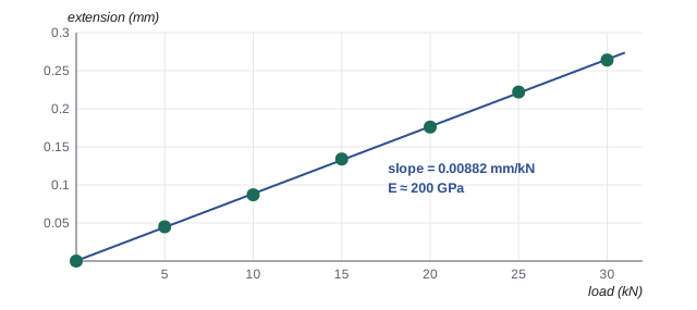
np.polyfit(x, y, 1) finds the straight line that best fits data in the least-squares sense (the method you met in MATH-125). For a tensile test, the slope of extension against load gives the stiffness, and from it Young's modulus.
Worked problem
Young's modulus by least squares
The test bar is 12 mm in diameter with a 200 mm gauge length. Fit a line to the data and compute E.
Show solution
import numpy as np load_kN = np.array([0, 5, 10, 15, 20, 25, 30]) ext_mm = np.array([0.000, 0.045, 0.087, 0.134, 0.176, 0.222, 0.264]) slope, intercept = np.polyfit(load_kN, ext_mm, 1) # mm per kN area_mm2 = np.pi * 12 ** 2 / 4 gauge_mm = 200 E_MPa = (1000 / area_mm2) / (slope / gauge_mm) # stress / strain for 1 kN print(f"slope = {slope:.6f} mm/kN, intercept = {intercept:.5f} mm") print(f"E = {E_MPa / 1000:.1f} GPa")- Output: slope = 0.008821 mm/kN, intercept = 0.00025 mm; E = 200.5 GPa.
- Check: 1 kN gives a stress of \(1000/113.1 = 8.84\) MPa and a strain of \(0.008821/200 = 4.41 \times 10^{-5}\); the ratio is \(2.00 \times 10^5\) MPa.
Answer: E ≈ 200 GPa, as expected for steel. The tiny intercept (0.00025 mm) confirms the data pass almost through the origin; a large intercept would suggest slack in the grips or a zero error
Integrating measured data
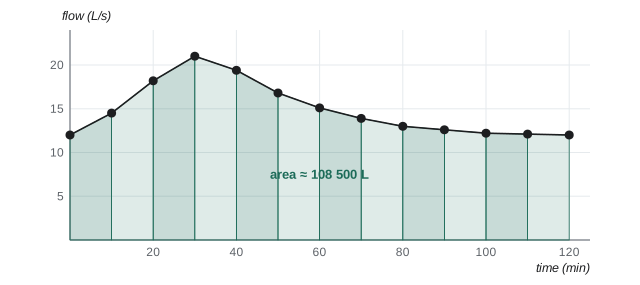
Many engineering quantities are integrals of measured rates: volume from flow rate, energy from power, impulse from force. With data at discrete times, the trapezoidal rule (MATH-100, Lesson 5) approximates the integral by summing trapezoids between readings.
Worked problem
Storm volume from flow readings
A sewer flow meter records these flows (L/s) every 10 minutes for 2 hours: 12.0, 14.5, 18.2, 21.0, 19.4, 16.8, 15.1, 13.9, 13.0, 12.6, 12.2, 12.1, 12.0. Find the total volume.
Show solution
import numpy as np flow_Ls = [12.0, 14.5, 18.2, 21.0, 19.4, 16.8, 15.1, 13.9, 13.0, 12.6, 12.2, 12.1, 12.0] t_min = np.arange(0, 121, 10) # 0, 10, ..., 120 # By hand-coded loop volume_L = 0 for i in range(len(flow_Ls) - 1): volume_L += (flow_Ls[i] + flow_Ls[i + 1]) / 2 * 10 * 60 # 10 min = 600 s # With NumPy volume_np = np.trapezoid(flow_Ls, t_min * 60) print(volume_L, volume_np)- Output: 108480.0 108480.0.
Answer: About 108 500 L, or 108.5 m³. The time had to be converted to seconds because the flow is in litres per second; unit consistency matters as much in code as on paper. (np.trapezoid is the name in NumPy 2.0 and later; older versions call it np.trapz.)
Solving linear systems
Systems of linear equations appear everywhere in engineering: truss and frame analysis, circuit analysis, heat flow, least squares. np.linalg.solve solves \(A\mathbf{x} = \mathbf{b}\) directly and reliably.
Worked problem
The three-cable problem in one line
In ENGG-130, Lesson 2, a 2.00 kN load hung from cables to B(3, −2, 6), C(−6, −3, 6) and D(0, 8, 6). The equilibrium equations were solved by substitution. Solve them with NumPy.
Show solution
- Each column of \(A\) is a cable's unit vector; \(\mathbf{b}\) is the load the cables must balance.
import numpy as np A = np.array([[ 3/7, -6/9, 0/10], [-2/7, -3/9, 8/10], [ 6/7, 6/9, 6/10]]) b = np.array([0, 0, 2000]) T = np.linalg.solve(A, b) print(T) print(A @ T) # check: should reproduce b- Output: [1204.30107527 774.19354839 752.68817204], then the check, which reproduces [0, 0, 2000] to within about 10⁻¹³ (rounding).
Answer: T_B = 1204 N, T_C = 774 N, T_D = 753 N, matching the hand solution. The @ operator is matrix multiplication; multiplying back to recover b is a quick, essential check
The same few lines solve systems of hundreds or thousands of equations, which is exactly what structural analysis software does when it analyzes a building frame. You now understand, in principle, what happens inside those programs.
Plotting
Matplotlib is the standard plotting library. A basic plot takes a handful of lines; always label axes with units and add a title or legend so the plot can stand on its own in a report (Lesson 4 of ENGG-160).
import numpy as np
import matplotlib.pyplot as plt

load_kN = np.array([0, 5, 10, 15, 20, 25, 30])
ext_mm = np.array([0.000, 0.045, 0.087, 0.134, 0.176, 0.222, 0.264])
slope, intercept = np.polyfit(load_kN, ext_mm, 1)

plt.plot(load_kN, ext_mm, "o", label="test data")
plt.plot(load_kN, slope * load_kN + intercept, "-", label="least-squares fit")
plt.xlabel("Load (kN)")
plt.ylabel("Extension (mm)")
plt.legend()
plt.savefig("tensile.png", dpi=150)      # or plt.show() to open a window
Simulation: Euler's method
Many engineering systems are described by differential equations: a tank draining, a beam vibrating, a circuit charging, a part cooling. When there is no neat formula for the solution, or even when there is, a program can step forward in time. Euler's method is the simplest scheme: if \(dy/dt = f(t, y)\), then over a small step \(\Delta t\), \(y_{new} = y + f(t, y)\,\Delta t\).
Worked problem
Cooling a casting
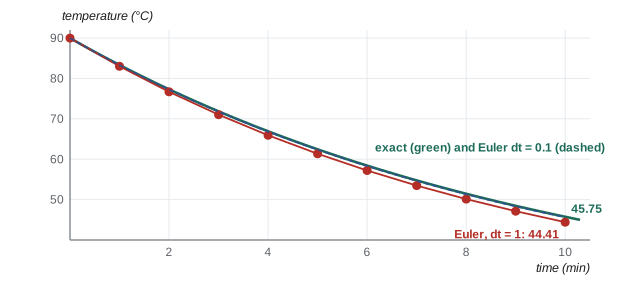
A casting at 90 °C cools in air at 20 °C according to Newton's law of cooling, \(dT/dt = -k(T - 20)\), with \(k = 0.1\) per minute. Estimate the temperature after 10 minutes with Euler steps of 1 minute and 0.1 minute, and compare with the exact solution \(T = 20 + 70e^{-kt}\).
Show solution
import math def euler_cooling(T0, T_air, k, t_end, dt): T = T0 steps = round(t_end / dt) for _ in range(steps): T = T + (-k * (T - T_air)) * dt return T exact = 20 + 70 * math.exp(-0.1 * 10) for dt in (1.0, 0.1): T = euler_cooling(90, 20, 0.1, 10, dt) print(f"dt = {dt}: {T:.2f} C (error {T - exact:+.2f})") print(f"exact: {exact:.2f} C")- Output: dt = 1.0: 44.41 C (error −1.34); dt = 0.1: 45.62 C (error −0.13); exact: 45.75 C.
Answer: About 45.8 °C exactly; Euler gives 44.4 °C with 1-minute steps and 45.6 °C with 0.1-minute steps. Ten times smaller steps cut the error about ten times, the signature of a first-order method. Production simulations use higher-order methods (SciPy's solve_ivp, for example) that are far more accurate for the same effort
Where to go next
You now have the core of programming: values and types, decisions, loops, functions, collections, files and numerical libraries. From here, engineers typically add SciPy (optimization, integration, differential equations, signal processing), pandas (tables of data, like a programmable spreadsheet), and domain tools for their discipline. The habits matter more than the libraries: plan before coding, work in small steps, name things clearly with units, write functions with docstrings, test against hand calculations, and treat every result with an engineer's scepticism until it has been checked.
Common mistakes
MistakeOff-by-one indexing: using a[len(a)] or expecting a[1] to be the first item.
InsteadIndexes run from 0 to len(a) − 1; a[-1] is the last item.
MistakeForgetting that values read from files are strings.
InsteadConvert with float() or int(); skip header rows first.
MistakeWriting Python loops over large arrays of numbers.
InsteadUse NumPy whole-array operations: shorter, clearer and much faster.
MistakeMixing time units when integrating rates (minutes with L/s).
InsteadConvert to a consistent system before integrating, and check the units of the result.
MistakeTrusting np.linalg.solve output without checking.
InsteadMultiply back (A @ x) and compare with b; compare with a hand solution for a small case.
MistakeUsing a large Euler step and accepting the result.
InsteadHalve the step and rerun; if the answer changes noticeably, the step is too large.
Summary and key terms
- Lists hold ordered data; indexes start at 0, negative indexes count from the end, and slices stop before the stop index.
- List comprehensions transform and filter lists in one line; dictionaries look up values by key.
- Use with open() and the csv module to read and write files; convert text fields to numbers and skip headers.
- NumPy arrays support fast, vectorized arithmetic, statistics and boolean selection.
- np.polyfit fits lines and curves by least squares; np.trapezoid integrates sampled data; np.linalg.solve solves linear systems.
- Matplotlib produces plots; label axes with units.
- Euler's method steps a differential equation forward in time; its error shrinks in proportion to the step size.
- List
- An ordered, changeable collection of values.
- Index
- The position of an item in a sequence, starting at 0.
- Slice
- A sub-sequence a[start:stop], including start and excluding stop.
- List comprehension
- A one-line expression that builds a list from another sequence.
- Dictionary
- A collection that maps keys to values.
- CSV
- Comma-separated values, a plain-text table format.
- NumPy array
- A fixed-type block of numbers supporting fast whole-array operations.
- Vectorization
- Applying an operation to a whole array at once instead of looping.
- Least squares
- Fitting a model by minimizing the sum of squared differences from data.
- Trapezoidal rule
- Approximating an integral by summing trapezoids between data points.
- Euler's method
- A first-order scheme for stepping a differential equation forward in time.
Practice problems
Work each problem on paper first, then reveal the answer to check.
Given a = [4, 8, 15, 16, 23, 42], what are a[1], a[-2], a[2:4] and a[::2]?
Show answer
8; 23; [15, 16]; [4, 15, 23] (every second item).
Write a comprehension that converts temperatures_C = [−10, 0, 25] to Fahrenheit.
Show answer
[c * 9 / 5 + 32 for c in temperatures_C] gives [14.0, 32.0, 77.0].
Create a dictionary of yield strengths (MPa): "300W": 300, "350W": 350, and print the value for "350W".
Show answer
fy = {"300W": 300, "350W": 350}; print(fy["350W"]) prints 350. (300W and 350W are Canadian structural steel grade designations.)
A CSV file has a header line and then lines like 2026-03-01,14.2. Write code to read the second column into a list of floats.
Show answer
with open(name, newline="") as f: r = csv.reader(f); next(r); values = [float(row[1]) for row in r].
With NumPy, compute the kinetic energy ½mv² for m = 1500 kg and speeds v = [10, 20, 30] m/s in one line.
Show answer
0.5 * 1500 * np.array([10, 20, 30]) ** 2 gives [75000, 300000, 675000] J.
Fit a line to x = [1, 2, 3, 4], y = [2.1, 3.9, 6.2, 7.8]. What slope and intercept do you expect roughly?
Show answer
np.polyfit gives slope 1.94 and intercept 0.15 (y ≈ 1.94x + 0.15).
Power readings (kW) every 15 minutes for an hour are 40, 52, 60, 55, 45. Use the trapezoidal rule to find the energy in kWh.
Show answer
Δt = 0.25 h. Energy = 0.25 × [(40 + 52)/2 + (52 + 60)/2 + (60 + 55)/2 + (55 + 45)/2] = 0.25 × 209.5 = 52.4 kWh.
Solve with NumPy: 2x + y = 5 and x − 3y = −1.
Show answer
np.linalg.solve([[2, 1], [1, -3]], [5, -1]) gives x = 2, y = 1.
In the cooling example, what would Euler with dt = 0.5 min give, roughly?
Show answer
The error scales with dt, so about −0.67: roughly 45.1 °C. (Running it gives 45.09 °C.)
Why is np.trapezoid(flow, t) wrong if t is in minutes and flow in L/s?
Show answer
The result would be in L·min/s, 60 times too small to be litres. Multiply t by 60 (or the result by 60) to get litres.
Lesson quiz · 5 questions
Score 60% or more to complete this lesson.
Create a free account to save your progress, take quizzes and earn a certificate.