
ELE-480 · Lesson 4 of 12 · 21 min
Overcurrent relays and time-current curves
Overcurrent protection is the oldest, cheapest and most widely used form of protection. Every one of Lincoln Road's four feeders is protected by overcurrent relays, the recloser and fuses on feeder F2 are overcurrent devices, and the transformer's backup protection is overcurrent too. The idea is simple: a fault draws much more current than a load, so trip when the current exceeds a threshold. The art lies in choosing the threshold and the time delay so that each device protects its own zone, stays quiet for load and for faults that a device closer to them should clear, and backs up its neighbours. This lesson covers the relay elements and their curves; lesson 5 applies them to the coordination of a whole feeder.
Instantaneous and time-overcurrent elements
An overcurrent relay offers two basic elements. The instantaneous element, device 50, operates as soon as the current exceeds its pickup setting, with no intentional delay; a numerical relay's instantaneous element typically operates in about a cycle. A definite-time element is an instantaneous element followed by a fixed timer. The time-overcurrent element, device 51, operates after a delay that decreases as the current increases, following an inverse-time curve. Each element exists for phase currents (50P, 51P), for the residual or ground current, the sum of the three phase currents (50N, 51N or 50G, 51G), and in numerical relays for negative-sequence current (50Q, 51Q).
The inverse characteristic suits faults on radial systems well. A fault close to the source draws a large current and is cleared quickly; a fault far away draws less current and is cleared more slowly, which leaves time for devices closer to that fault to act first. The shape of the curve, how steeply the time falls as current rises, is chosen to match the devices it must coordinate with.
Standard curves
Electromechanical induction-disc relays produced their inverse characteristics from the physics of the disc, and each manufacturer's curves were slightly different. To allow numerical relays to reproduce them and to make coordination between makers practical, IEEE C37.112 defines a standard equation for inverse-time characteristics, and IEC 60255-151 defines a similar family used widely outside North America. In the IEEE form the operating time t, for a current that is M times the pickup, is:
TD is the time dial, which scales the curve up or down, and A, B and p are constants that set its shape. The IEC form is t = TMS × k/(M^α − 1), with a time multiplier setting TMS. Many relays label the IEEE curves U1 to U5.
| Curve | A | B | p |
|---|---|---|---|
| U1 moderately inverse | 0.0515 | 0.1140 | 0.02 |
| U2 inverse | 5.95 | 0.180 | 2.0 |
| U3 very inverse | 3.88 | 0.0963 | 2.0 |
| U4 extremely inverse | 5.67 | 0.0352 | 2.0 |
| U5 short-time inverse | 0.00342 | 0.00262 | 0.02 |
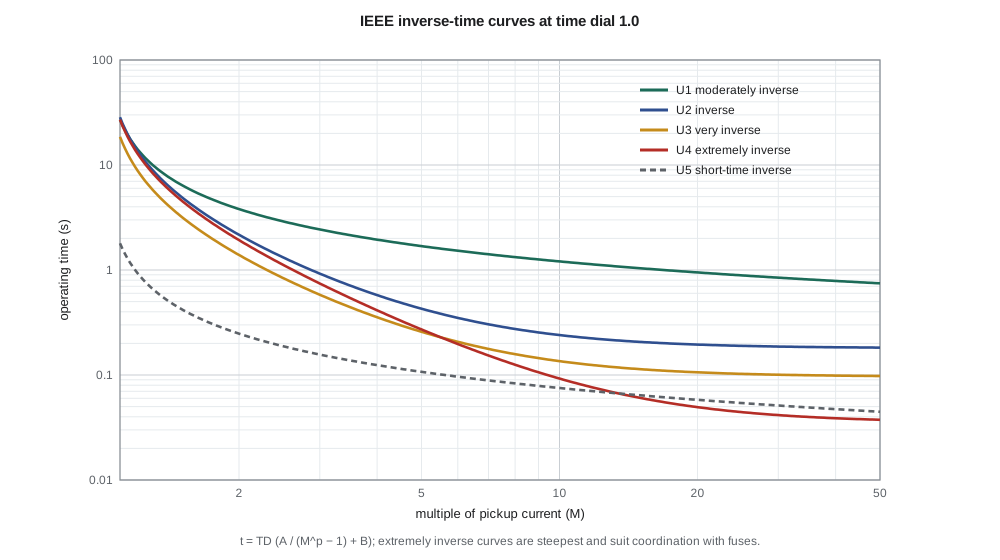
# Inverse-time overcurrent curves: IEEE (C37.112) and IEC (60255-151) forms
IEEE = {'U1 moderately inverse': (0.0515, 0.1140, 0.02), 'U2 inverse': (5.95, 0.180, 2.0),
        'U3 very inverse': (3.88, 0.0963, 2.0), 'U4 extremely inverse': (5.67, 0.0352, 2.0),
        'U5 short-time inverse': (0.00342, 0.00262, 0.02)}
IEC = {'C1 standard inverse': (0.14, 0.02), 'C2 very inverse': (13.5, 1.0),
       'C3 extremely inverse': (80.0, 2.0), 'C4 long-time inverse': (120.0, 1.0)}
def t_ieee(curve, td, M):
    A, B, p = IEEE[curve]; return td*(A/(M**p - 1) + B)
def t_iec(curve, tms, M):
    k, a = IEC[curve]; return tms*k/(M**a - 1)
print("operating time (s) at multiples of pickup, IEEE time dial 1.0 / IEC TMS 0.1")
print("curve                       M=2     M=5    M=10    M=20")
for c in IEEE: print(f"{c:26s}" + "".join(f"{t_ieee(c, 1.0, M):8.3f}" for M in (2, 5, 10, 20)))
for c in IEC:  print(f"{c:26s}" + "".join(f"{t_iec(c, 0.1, M):8.3f}" for M in (2, 5, 10, 20)))

# Feeder F2: CT 600/5, pickup 2.4 A secondary (288 A primary), U4 curve.
pickup = 2.4*120
for I, tgt in ((5865, None), (1280, 0.65)):
    M = I/pickup
    if tgt is None:
        print(f"\nI = {I} A is {M:.1f} x pickup")
        continue
    td = tgt/(5.67/(M**2 - 1) + 0.0352)
    print(f"I = {I} A is {M:.2f} x pickup; time dial for {tgt} s: {td:.2f}")
td = 2.0
for I in (600, 1280, 2500, 5865):
print(f"TD {td}: {I:5d} A -> {t_ieee('U4 extremely inverse', td, I/pickup):6.2f} s")operating time (s) at multiples of pickup, IEEE time dial 1.0 / IEC TMS 0.1 curve M=2 M=5 M=10 M=20 U1 moderately inverse 3.803 1.688 1.207 0.948 U2 inverse 2.163 0.428 0.240 0.195 U3 very inverse 1.390 0.258 0.135 0.106 U4 extremely inverse 1.925 0.271 0.092 0.049 U5 short-time inverse 0.248 0.107 0.075 0.058 C1 standard inverse 1.003 0.428 0.297 0.227 C2 very inverse 1.350 0.338 0.150 0.071 C3 extremely inverse 2.667 0.333 0.081 0.020 C4 long-time inverse 12.000 3.000 1.333 0.632 I = 5865 A is 20.4 x pickup I = 1280 A is 4.44 x pickup; time dial for 0.65 s: 1.93 TD 2.0: 600 A -> 3.47 s TD 2.0: 1280 A -> 0.68 s TD 2.0: 2500 A -> 0.22 s TD 2.0: 5865 A -> 0.10 s
The table from the program shows the different personalities of the curves. At twice pickup the moderately inverse curve takes 3.8 s and the extremely inverse 1.9 s; at twenty times pickup the moderately inverse still takes 0.95 s while the extremely inverse takes 0.05 s. Moderately inverse curves suit systems where the fault current changes little along the line, such as transmission and subtransmission networks with strong sources. Very and extremely inverse curves suit distribution feeders, where the current falls sharply with distance, and they match the steep curves of fuses, which behave roughly like an I²t characteristic. The short-time inverse curve is used where fast operation is wanted with a little time grading.
Choosing the pickup
The pickup must be above the highest current the relay will see in normal and emergency operation, and below the smallest fault current it must detect, with margins at both ends. For a phase element the upper limit comes from load. Feeder F2's peak load is about 190 A, but after a long outage, when the feeder is re-energized, thermostats, water heaters and motors all start together and the current can exceed the normal peak for several seconds or minutes. This cold-load pickup is the reason phase pickups are usually set at 1.5 to 2 times maximum load, or the relay's settings are temporarily raised after a re-energization.
Nadine and Leo choose a phase pickup of 288 A primary, 1.5 times the 190 A peak load, which with the 600:5 CT is 2.4 A secondary. The lower limit is the minimum fault current at the end of the zone, which lesson 2 found to be about 1.2 kA for a line-to-line fault at the end of F2 under minimum conditions. That fault is more than four times pickup, comfortably above the factor of two that many utilities require so that the relay operates reliably and on a steep part of its curve.
Ground elements measure the residual current, which is near zero in a balanced system, so they can be set well below load current. Their lower limit comes from the normal unbalance of single-phase loads on a distribution feeder, which produces some residual current all the time; a pickup of 30 to 50 % of the phase pickup is common on four-wire multigrounded feeders. That sensitivity is what lets ground elements see the resistive ground faults that phase elements miss.
Choosing the curve and time dial
With the pickup chosen, the time dial is set so that the relay operates in a chosen time at a chosen current, usually so that it coordinates with the next device downstream. As a first pass, before looking at the recloser, Leo picks the extremely inverse curve and asks for 0.65 s for the 1.28 kA ground fault at 12 km, which gives a time dial of about 1.9; he rounds it to 2.0. The program shows the resulting times: 3.5 s at 600 A, 0.68 s at 1280 A, 0.22 s at 2500 A and 0.10 s for the largest fault at the bus. Lesson 5 will show that this first setting is too fast to coordinate with the recloser, and it will change.
A useful habit is to compute the multiple of pickup before reading any curve: 5865 A is 20.4 times the 288 A pickup. Most relays define their curves up to about 20 or 30 times pickup and become definite-time beyond, so the very highest currents may be treated as the curve's limiting value.
Instantaneous elements and overreach
An instantaneous element clears close-in faults quickly, which reduces damage and arc flash energy at the substation. But it has no time delay to coordinate with, so it must be set high enough that it does not operate for faults in the next zone downstream. The usual rule sets it at 1.25 to 1.5 times the maximum fault current at the far end of its own zone or at the next device. On a feeder with a recloser, the instantaneous element must not see faults beyond the recloser, so its pickup is set above the maximum fault at the recloser location, and it covers only the first part of the feeder.
A second effect also has to be allowed for: transient overreach. The DC offset of a fault current makes the first peaks larger than the symmetrical current, and an instantaneous element that responded to peaks would operate for faults slightly beyond its setting. Numerical relays filter out the DC component and respond to the fundamental, so their transient overreach is small, but margins in the setting rule cover it anyway.
Reset characteristics
An induction disc rotates toward its trip contact while the current is above pickup and turns back slowly under its spring when the current drops. If a fault is cleared by a downstream device and then a recloser recloses into it, the disc has not fully reset, so the upstream relay trips sooner on the second shot than it did on the first. Numerical relays offer an electromechanical reset that imitates this behaviour, or an instantaneous reset that starts every timing from zero. When a relay must coordinate with a recloser that recloses quickly, the reset choice affects whether the relay ratchets toward a trip during the reclose sequence, and the two devices must be checked together.
Directional and voltage-restrained variants
Plain overcurrent relays respond to current magnitude only. Where fault current can flow in either direction through the relay location, on loops, parallel lines and feeders with distributed generation, a directional element supervises the overcurrent element so that it operates only for faults in one direction; lesson 6 covers it. At generator terminals, where the fault current of a machine decays below its full-load current within a second or two, voltage-restrained or voltage-controlled overcurrent elements lower their pickup when the voltage collapses, so that the relay still sees a sustained fault.
Worked problem
Setting a ground time-overcurrent element
Feeder F2's ground element (51N) uses the same 600:5 CTs. The feeder carries up to about 30 A of residual current from normal unbalance. The smallest ground fault it must detect is about 510 A, a 20 Ω fault at 18 km under minimum conditions. Choose a pickup and check the margin.
Show solution
- Pickup must exceed normal residual current with margin: 4 × 30 = 120 A gives room for unbalance growth.
- \[120\ \text{A} / 120 = 1.0\ \text{A secondary}\]
- \[M = \frac{510}{120} = 4.3\]
- A multiple of 4.3 is well above the factor of about 2 wanted for reliable operation, so 120 A is suitable; the time dial is chosen in lesson 5.
Answer: A pickup of 120 A (1.0 A secondary) sees the 510 A resistive fault at more than four times pickup.
Common mistakes
MistakeSetting the phase pickup just above peak load.
InsteadAllow for cold-load pickup and emergency loading: 1.5 to 2 times peak load is common.
MistakeReading a curve without first computing the multiple of pickup.
InsteadAll standard curves are defined in multiples of pickup, not amperes.
MistakeSetting an instantaneous element to cover the whole feeder.
InsteadIt would trip for faults beyond the downstream device; set it above the maximum fault there.
MistakeIgnoring the relay's reset characteristic on reclosing feeders.
InsteadAn electromechanical-style reset can let the relay ratchet toward a trip during a reclose sequence.
Summary and key terms
- Instantaneous (50) elements trip without intentional delay; time-overcurrent (51) elements follow inverse curves.
- IEEE C37.112 curves follow t = TD(A/(M^p − 1) + B); IEC curves follow t = TMS·k/(M^α − 1).
- Extremely inverse curves suit distribution and fuses; moderately inverse suits strong networks.
- Phase pickup sits above load and cold-load pickup and below the minimum fault with a margin.
- Ground elements measure residual current and can be set well below load current.
- Instantaneous elements are set above the maximum fault at the next device to avoid overreach.
- Reset behaviour matters when relays coordinate with reclosers.
- Pickup
- The smallest current at which an element starts to operate.
- Time dial (TD)
- The setting that scales an inverse-time curve up or down.
- Multiple of pickup (M)
- The measured current divided by the pickup current.
- Cold-load pickup
- The high current drawn when a feeder is re-energized after a long outage.
- Residual current
- The sum of the three phase currents, equal to 3I₀.
- Transient overreach
- Operation of an instantaneous element for a fault beyond its setting because of DC offset.
- Definite-time element
- An overcurrent element with a fixed time delay independent of current.
Practice problems
Work each problem on paper first, then reveal the answer to check.
A U4 relay has a pickup of 300 A and TD 2.0. How long does it take at 3000 A?
Show answer
M = 10: 2.0 × (5.67/99 + 0.0352) ≈ 0.19 s.
Why are extremely inverse curves chosen to coordinate with fuses?
Show answer
Their shape follows the steep I²t characteristic of fuses.
Peak load is 220 A. Suggest a phase pickup range.
Show answer
About 330 to 440 A (1.5 to 2 times).
Why can a ground element be set below load current?
Show answer
It measures residual current, which is near zero for balanced load.
The maximum fault at the recloser is 3.4 kA. Where should the feeder's instantaneous element be set?
Show answer
Above about 4.3 to 5.1 kA (1.25 to 1.5 times).
What is the multiple of pickup for 5865 A with a 288 A pickup?
Show answer
About 20.4.
Lesson quiz · 5 questions
Score 60% or more to complete this lesson.
Create a free account to save your progress, take quizzes and earn a certificate.