Propagation and channel models

ELE-350 built the TLR-1 link budget from free-space loss, a two-ray breakpoint, shadowing allowances and Rayleigh fading. Those tools served well for a 45 m link across an intersection and a 600 m link between cabinets on mast arms, where the antennas could see each other or nearly so. The cellular backhaul of TLR-2 is a different kind of link. Its far end is a cell site that Cedarline does not control, several kilometres away, beyond buildings and trees, chosen by a carrier for coverage of phones, not traffic cabinets. Whether a given cabinet will connect reliably is a question for empirical propagation models, the subject of this lesson, followed by a site survey with a real module.

Why empirical models

Free-space loss assumes a clear path. Real paths in cities pass over and between buildings, are diffracted by rooftops and edges, reflected by walls and the ground, and absorbed by foliage. The two-ray model of ELE-350 adds one ground reflection and predicts a loss that rises at 40 dB per decade beyond the breakpoint distance. Measured urban paths often fall somewhere between, with a path-loss exponent n of about 3 to 4 and large variations about the median. Rather than model every building, engineers fit simple formulas to many measurements. The formulas are valid only within the conditions of the measurements, but within those limits they predict median path loss well enough to plan networks and to judge whether a fixed installation is likely to work.

The log-distance model, used in ELE-350, expresses this with a reference loss at distance d₀ and an exponent n: PL(d) = PL(d₀) + 10n log₁₀(d/d₀) + X_σ, where X_σ is a log-normal shadowing term with standard deviation σ of typically 6 to 10 dB. The Okumura–Hata model is the best known of the empirical models that predict PL(d₀) and n from frequency, antenna heights and the type of area.

The Okumura–Hata model

Okumura measured path loss in and around Tokyo in the 1960s and published curves; Hata fitted formulas to them. For a small or medium city, with frequency f in megahertz (valid roughly from 150 to 1500 MHz), base-station antenna height h_b of 30 to 200 m, mobile antenna height h_m of 1 to 10 m and distance d of 1 to 20 km, the median path loss is:

The terms tell the story. Loss rises with frequency, at about 26 dB per decade. It falls as the base-station antenna is raised and, through a(h_m), as the mobile antenna is raised. The distance exponent is 44.9 − 6.55 log₁₀ h_b, about 35 dB per decade for a 30 m site: a path-loss exponent of 3.5. Other versions of the model add corrections for large cities, suburbs and open rural areas. The COST-231 extension, developed in Europe for the 1800 MHz band, changes the constants to cover 1500 to 2000 MHz.

import math

# Okumura-Hata median path loss, small or medium city (valid about 150-1500 MHz, 1-20 km)
def hata(f_mhz, d_km, hb, hm):
    ahm = (1.1*math.log10(f_mhz) - 0.7)*hm - (1.56*math.log10(f_mhz) - 0.8)
    return 69.55 + 26.16*math.log10(f_mhz) - 13.82*math.log10(hb) - ahm + (44.9 - 6.55*math.log10(hb))*math.log10(d_km)
# COST-231 extension for 1500-2000 MHz (C = 0 dB for medium city and suburban areas)
def cost231(f_mhz, d_km, hb, hm, C=0.0):
    ahm = (1.1*math.log10(f_mhz) - 0.7)*hm - (1.56*math.log10(f_mhz) - 0.8)
    return 46.3 + 33.9*math.log10(f_mhz) - 13.82*math.log10(hb) - ahm + (44.9 - 6.55*math.log10(hb))*math.log10(d_km) + C
def fspl(f_mhz, d_km): return 32.45 + 20*math.log10(f_mhz) + 20*math.log10(d_km)

hb, hm = 30.0, 6.0          # cell-site antenna height, cabinet antenna on the mast arm (m)
print(" d (km)  FSPL 739   Hata 739   Hata 881   COST-231 1960 MHz")
for d in (1, 2, 3, 5, 8):
    print(f"  {d:4.0f}    {fspl(739, d):6.1f}    {hata(739, d, hb, hm):6.1f}     {hata(881, d, hb, hm):6.1f}      {cost231(1960, d, hb, hm):6.1f}")
# Effect of mounting height at the cabinet
for h in (1.5, 3.0, 6.0):
    print(f"  cabinet antenna at {h} m: Hata 739 MHz at 3 km = {hata(739, 3, hb, h):6.1f} dB")

# Knife-edge diffraction loss (ITU-R P.526 approximation)
def knife(v): return 0.0 if v <= -0.78 else 6.9 + 20*math.log10(math.sqrt((v - 0.1)**2 + 1) + v - 0.1)
lam = 3e8/739e6; d1, d2 = 2200.0, 800.0
for h in (-5.0, 0.0, 5.0, 10.0):         # obstruction height above the line of sight, m
    v = h*math.sqrt(2*(d1 + d2)/(lam*d1*d2))
    print(f"  building edge {h:+5.1f} m above the path: v = {v:5.2f}, extra loss {knife(v):4.1f} dB")

# Fade margin for coverage reliability at the cabinet with log-normal shadowing
def qinv(p):
    lo, hi = -8.0, 8.0
    for _ in range(80):
        m = (lo + hi)/2
        if 0.5*math.erfc(m/math.sqrt(2)) > p: lo = m
        else: hi = m
    return m
for rel in (0.90, 0.95, 0.99):
    print(f"  {rel*100:.0f} % location reliability with sigma 8 dB: margin {qinv(1 - rel)*8:4.1f} dB")

 d (km)  FSPL 739   Hata 739   Hata 881   COST-231 1960 MHz
     1      89.8     113.1      114.7       124.3
     2      95.8     123.7      125.3       134.9
     3      99.4     129.9      131.5       141.1
     5     103.8     137.7      139.4       148.9
     8     107.9     144.9      146.5       156.1
  cabinet antenna at 1.5 m: Hata 739 MHz at 3 km =  141.0 dB
  cabinet antenna at 3.0 m: Hata 739 MHz at 3 km =  137.3 dB
  cabinet antenna at 6.0 m: Hata 739 MHz at 3 km =  129.9 dB
  building edge  -5.0 m above the path: v = -0.46, extra loss  2.3 dB
  building edge  +0.0 m above the path: v =  0.00, extra loss  6.0 dB
  building edge  +5.0 m above the path: v =  0.46, extra loss  9.9 dB
  building edge +10.0 m above the path: v =  0.92, extra loss 13.4 dB
  90 % location reliability with sigma 8 dB: margin 10.3 dB
  95 % location reliability with sigma 8 dB: margin 13.2 dB
  99 % location reliability with sigma 8 dB: margin 18.6 dB

The program evaluates the models for a cabinet antenna at 6 m, the height of the mast arm, and a cell site 30 m high. At 3 km, Hata gives 129.9 dB at 739 MHz (LTE band 12 or 13) and 131.5 dB at 881 MHz (band 5), about 30 dB more than free space; COST-231 gives 141.1 dB at 1960 MHz (band 2 or 25). Low bands are worth more than 10 dB at the same distance, which is why the low-power cellular standards favour them and why the cabinet module should be allowed to choose band 12, 13 or 5 where the carrier offers it.

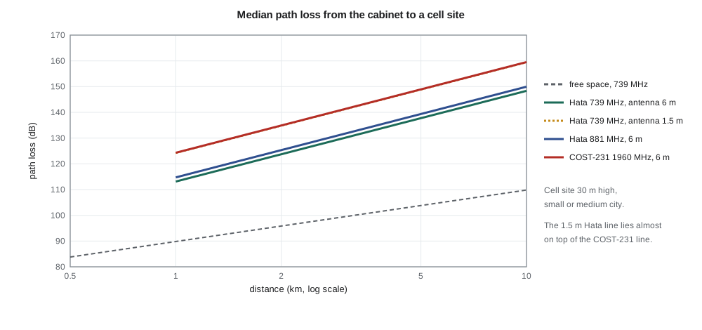
The cabinet antenna height matters a great deal. At 3 km and 739 MHz, lowering the antenna from 6 m to 1.5 m, the height of an antenna on the cabinet roof itself, raises the loss from 129.9 to 141.0 dB. Amara had planned a roof antenna for simplicity; the model persuades her to specify a mast-arm mount where the cabinet is near a signal pole, with the cable loss of lesson 8 a small price.

Diffraction

A building between the cabinet and the cell site blocks part of the first Fresnel zone, the ellipsoid around the direct path within which most of the energy travels. ELE-350 computed the zone's radius; here we estimate the extra loss when an obstacle intrudes. Treating the obstacle as a sharp edge, the knife-edge diffraction parameter v combines the edge height h above the direct path with the distances d₁ and d₂ to each end.

The approximation, from ITU-R Recommendation P.526, applies for v greater than about −0.78; below that the loss is negligible. A building edge exactly on the line of sight (v = 0) costs 6 dB, because half the Fresnel zone is blocked. With the edge 5 m above the line, 2.2 km from the cabinet and 0.8 km from the site, the program finds v = 0.46 and 9.9 dB of extra loss; at 10 m, 13.4 dB. Even an edge 5 m below the line costs 2.3 dB, because it still obstructs part of the zone. Hata's formula already includes typical urban diffraction in its median, so the knife-edge estimate is used for a specific known obstruction, such as a new building between a cabinet and its site, not added routinely.

Fading and fade margins

About the median, path loss varies in two ways. Shadowing changes slowly as the terminal moves past buildings and trees, and is modelled as log-normal with a standard deviation σ. Multipath fading changes over fractions of a wavelength as reflected waves add and cancel, and is modelled by Rayleigh or Rician statistics, as ELE-350 showed. For a fixed cabinet, multipath fading changes only when the surroundings move: passing trucks, opening garage doors, swaying trees. Shadowing, on the other hand, is fixed for a given cabinet: a cabinet in a deep shadow stays there.

Planners therefore choose a location reliability, the fraction of locations at the predicted distance where the link should work, and add a fade margin equal to the corresponding number of standard deviations. The program uses σ = 8 dB, typical for urban macrocells: 90 % of locations need a margin of 10.3 dB, 95 % need 13.2 dB and 99 % need 18.6 dB. Amara chooses 90 % for planning, the value carried into the capstone link budget, and relies on a site survey to find the cabinets in the unlucky 10 %, where a mast mount, a higher-gain antenna or a different carrier will be needed.

Building and enclosure penetration

Signals entering buildings lose typically 10 to 20 dB through walls and windows, more through metallized glass and concrete, which is why indoor coverage plans add a building penetration margin. For TLR-2 the corresponding penalty is the cabinet itself: a closed steel enclosure would add 20 dB or more, as lesson 8 noted, and an antenna inside a cabinet against its door is a common cause of failed installations elsewhere in the industry. With an external antenna the penalty disappears, but a nearby wall of the cabinet, a few centimetres from a roof antenna, still distorts the antenna pattern. The installation guide calls for the antenna at least 30 cm from vertical metal.

Coverage enhancement in LPWAN cellular

LTE-M and NB-IoT were designed to reach terminals in difficult places such as basements and meter closets. Their coverage-enhancement modes repeat each transmission many times, so that the receiver can combine the copies; each doubling of repetitions gains about 3 dB at the cost of airtime and energy. The design targets were a maximum coupling loss, the largest path loss between base station and device at which the link still works, of about 156 dB for LTE-M and about 164 dB for NB-IoT, compared with about 144 dB for ordinary LTE, though actual networks may configure fewer repetitions. For a cabinet whose margin is poor, these modes are a useful reserve, but every message then costs more energy and latency, and a cabinet that depends on deep coverage enhancement every day is better fixed with a better antenna position.

Models predict medians; sites decide. Before ordering hardware for the first city, Leo drives to twenty cabinets with an evaluation board for the cellular module and a mast-mounted antenna, and records received signal power and quality for each carrier. His results fall within about ±8 dB of the Hata prediction, consistent with the assumed σ, and two cabinets behind a hospital and a parking garage need mast mounts.