RF passive components and printed-circuit realization

The matching networks of lesson 3 used ideal inductors and capacitors. The parts that Leo solders onto the TLR-2 test boards are not ideal. A 10 pF capacitor in a 0402 package (1.0 × 0.5 mm) has a few tenths of a nanohenry of inductance in its electrodes and terminations; a 12 nH chip inductor has a fraction of a picofarad between its turns and a resistance that rises with frequency. The board itself adds inductance in every via and capacitance under every pad. At 915 MHz these parasitics shift a match by a few percent; at 2.4 GHz they can turn a capacitor into an inductor. This lesson describes how real passive parts behave at radio frequencies, how printed-circuit structures become circuit elements, and how filters, the passive circuits that most directly protect a receiver and clean up a transmitter, are designed and built.

Real capacitors

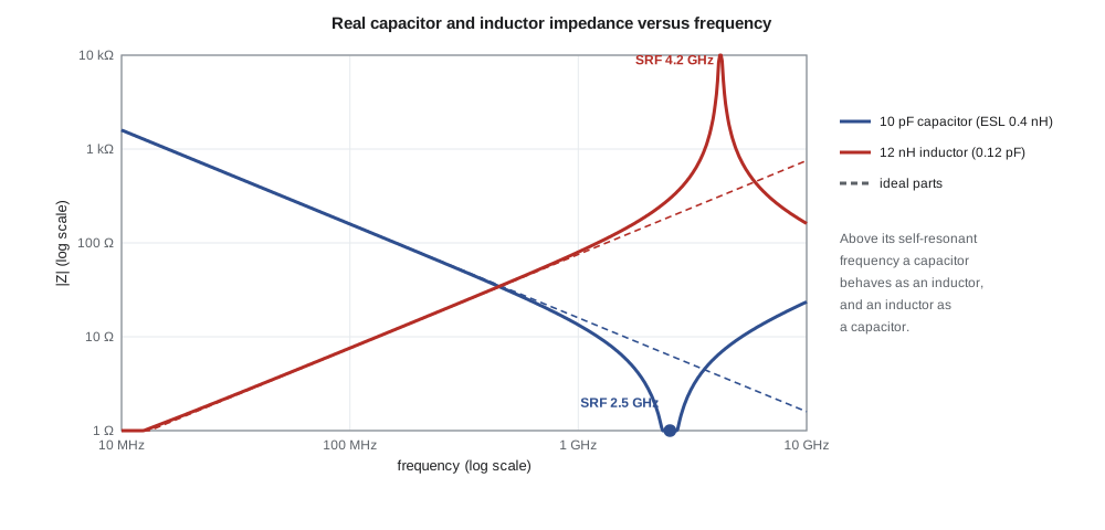
A surface-mount ceramic capacitor is modelled well up to a few gigahertz by its capacitance C in series with an equivalent series inductance (ESL) and an equivalent series resistance (ESR). The inductance comes from the current path through the electrodes and terminations and is set mainly by the package size and the way the part is mounted; for 0402 parts it is a few tenths of a nanohenry. The series combination resonates at the self-resonant frequency (SRF).

Below the SRF the part behaves as a capacitor whose effective capacitance rises as the inductance cancels part of its reactance; at the SRF its impedance falls to the ESR; above it the part is an inductor. A 10 pF capacitor with 0.4 nH of ESL resonates near 2.5 GHz. Used as a DC block or bypass, that is excellent: at its SRF it is the lowest impedance it can be. Used as a 10 pF element in a 2.44 GHz BLE match, it is useless, because its reactance there is nearly zero rather than −6.5 Ω. Radio-frequency capacitors therefore come with S-parameter files or equivalent-circuit models from the manufacturer, and the designer uses them in the simulation instead of ideal values.

The dielectric matters as much as the package. Class 1 ceramics such as C0G (NP0) have capacitance that hardly changes with temperature, voltage or age and very low loss, and are the only choice for matching networks, filters and oscillators. Class 2 ceramics such as X7R pack much more capacitance into a package, but their capacitance falls with applied DC voltage and with temperature, and their loss is higher; they are used for supply bypassing, not in signal paths.

Real inductors

A chip inductor has inductance L, a series resistance R that grows with frequency because of skin and proximity effects, and a parasitic capacitance between turns and terminals that resonates with L at its own SRF. Below the SRF the reactance rises faster than ωL as the capacitance takes effect; above it the part is capacitive. The quality factor Q = ωL/R rises with frequency at first, peaks, and then collapses as the SRF approaches.

Inductor construction sets both Q and SRF. Multilayer ceramic inductors are small and cheap but have Q of perhaps 10 to 30 at 1 GHz. Thin-film inductors are precise, with tolerances of ±0.1 nH, but have modest Q. Wire-wound ceramic-core chip inductors have the highest Q, often 40 to 80 at 1 GHz, and are used in low-noise amplifier inputs and power amplifier matches where loss counts. Air-core spring inductors have even higher Q but are hard to place by machine.

import math, cmath

# 1. Real capacitor and inductor (illustrative 0402 parts)
def cap_z(f, C, esl, esr): w = 2*math.pi*f; return esr + 1j*(w*esl - 1/(w*C))
def ind_z(f, L, Cpar, R0):
    w = 2*math.pi*f; R = R0 + 0.065*math.sqrt(f/1e6)   # winding loss grows with skin effect
    zl = R + 1j*w*L; return 1/(1/zl + 1j*w*Cpar)
C, esl, esr = 10e-12, 0.4e-9, 0.25
L, cpar, rl = 12e-9, 0.12e-12, 0.1
print(f"10 pF capacitor SRF {1/(2*math.pi*math.sqrt(esl*C))/1e9:.2f} GHz;  12 nH inductor SRF {1/(2*math.pi*math.sqrt(L*cpar))/1e9:.2f} GHz")
for f in (100e6, 915e6, 2.44e9, 4e9):
    zc = cap_z(f, C, esl, esr); zi = ind_z(f, L, cpar, rl)
    print(f"  {f/1e9:5.3f} GHz: capacitor {zc.real:5.2f}{zc.imag:+8.2f}j ohm   inductor {zi.real:7.1f}{zi.imag:+8.1f}j ohm  (Q {zi.imag/zi.real:5.1f})")

# 2. Via inductance (approximate formula, h and d in mm, result in nH)
def via_l(h, d): return 0.2*h*(math.log(4*h/d) + 1)
for h, d in ((1.6, 0.3), (0.2, 0.3)):
    print(f"via {h} mm long, {d} mm drill: about {via_l(h, d):.2f} nH -> {2*math.pi*915e6*via_l(h, d)*1e-9:.2f} ohm at 915 MHz")

# 3. Fifth-order 0.1 dB Chebyshev low-pass harmonic filter, cut-off 1.0 GHz, 50 ohm
n, ripple = 5, 0.1
beta = math.log(1/math.tanh(ripple/17.37)); gam = math.sinh(beta/(2*n))
a = [math.sin((2*k - 1)*math.pi/(2*n)) for k in range(1, n + 1)]
b = [gam**2 + math.sin(k*math.pi/n)**2 for k in range(1, n + 1)]
g = [2*a[0]/gam]
for k in range(1, n): g.append(4*a[k - 1]*a[k]/(b[k - 1]*g[k - 1]))
fc, R0 = 1.0e9, 50.0; wc = 2*math.pi*fc
parts = []
for k, gk in enumerate(g):            # shunt C first (Pi form), then series L, alternating
    if k % 2 == 0: parts.append(('C', gk/(R0*wc)))
    else: parts.append(('L', gk*R0/wc))
print("g values", " ".join(f"{x:.4f}" for x in g))
print("parts:", ", ".join(f"{t} {v*1e12:.2f} pF" if t == 'C' else f"{t} {v*1e9:.2f} nH" for t, v in parts))
def s21(f):
    w = 2*math.pi*f; A, B, Cc, D = 1, 0, 0, 1
    for t, v in parts:
        if t == 'C': M = (1, 0, 1j*w*v, 1)
        else: M = (1, 1j*w*v, 0, 1)
        A, B, Cc, D = A*M[0] + B*M[2], A*M[1] + B*M[3], Cc*M[0] + D*M[2], Cc*M[1] + D*M[3]
    return 2/(A + B/R0 + Cc*R0 + D)
for f in (0.915e9, 1.0e9, 1.83e9, 2.745e9, 3.66e9):
    print(f"  {f/1e9:5.3f} GHz  insertion loss {-20*math.log10(abs(s21(f))):6.2f} dB")

10 pF capacitor SRF 2.52 GHz;  12 nH inductor SRF 4.19 GHz
  0.100 GHz: capacitor  0.25 -158.90j ohm   inductor     0.8    +7.5j ohm  (Q  10.0)
  0.915 GHz: capacitor  0.25  -15.09j ohm   inductor     2.3   +72.4j ohm  (Q  31.8)
  2.440 GHz: capacitor  0.25   -0.39j ohm   inductor     7.6  +278.0j ohm  (Q  36.8)
  4.000 GHz: capacitor  0.25   +6.07j ohm   inductor   505.1 +3264.6j ohm  (Q   6.5)
via 1.6 mm long, 0.3 mm drill: about 1.30 nH -> 7.47 ohm at 915 MHz
via 0.2 mm long, 0.3 mm drill: about 0.08 nH -> 0.46 ohm at 915 MHz
g values 1.1468 1.3712 1.9750 1.3712 1.1468
parts: C 3.65 pF, L 10.91 nH, C 6.29 pF, L 10.91 nH, C 3.65 pF
  0.915 GHz  insertion loss   0.02 dB
  1.000 GHz  insertion loss   0.10 dB
  1.830 GHz  insertion loss  30.32 dB
  2.745 GHz  insertion loss  50.09 dB
  3.660 GHz  insertion loss  63.27 dB

The program's first part shows the effect. The 10 pF capacitor has a reactance of −15.1 Ω at 915 MHz, close to the ideal −17.4 Ω, but only −0.39 Ω at 2.44 GHz and +6.1 Ω at 4 GHz. The 12 nH inductor, whose resistance grows with the square root of frequency in this model, has a Q of about 32 at 915 MHz and an SRF near 4.2 GHz, above which it is useless. These are illustrative values of the kind found on 0402 data sheets.

The circuit board as a component

At radio frequencies the printed-circuit board is not a set of wires; it is a set of transmission lines, capacitors and inductors. ELE-360 designed the 50 Ω microstrip of TLR-1: a 0.38 mm trace on 0.2 mm FR-4 above a solid ground plane. TLR-2 keeps that stack-up, a four-layer board with the radio signals on the top layer and an unbroken ground plane on layer 2. The rules that follow from it are simple to state and easy to violate.

Every via that connects a component's ground terminal to the ground plane is a small inductor. A common estimate for a via of length h and diameter d, both in millimetres, is L ≈ 0.2h[ln(4h/d) + 1] nH. A via through the full 1.6 mm board has about 1.3 nH, 7.5 Ω at 915 MHz, which is comparable to the reactance of many matching parts. A via from the top layer to the layer-2 ground plane 0.2 mm below has only about 0.08 nH. Placing the ground plane on layer 2, close to the top, and using two or more vias for each ground connection keeps these inductances small. A shunt capacitor whose ground return goes through one long via is in fact a series resonant circuit.

Pads add capacitance. A component pad wider than the 0.38 mm trace is a short section of lower impedance, a small shunt capacitance; with large pads for 0603 parts on a thin dielectric this can be a few tenths of a picofarad. Designers remove the ground plane under large pads, or choose pad sizes close to the line width, to keep the line at 50 Ω. Bends are made with chamfered or curved corners to avoid the extra capacitance of a square corner.

For lines on the top layer where components need ground on either side, many designers use grounded coplanar waveguide (GCPW), a signal trace with ground copper on the same layer on both sides, stitched to the ground plane below with rows of vias. It confines the field better than microstrip, reduces coupling to nearby traces and makes shunt parts easy to ground, at the cost of a slightly harder impedance calculation. Priya uses GCPW for the telemetry front end on TLR-2 and microstrip for the longer runs to the antenna connectors.

Filters

Filters appear throughout TLR-2: the SAW filter in the cabinet receiver, the harmonic filter after the power amplifier, the low-pass filters in the transceiver's baseband and the duplexer inside the cellular module. Radio-frequency filters are specified by their passband, insertion loss and return loss in that band, and the rejection they provide at specific frequencies outside it.

Lumped LC filters are designed from normalized low-pass prototypes, tables of element values g₁ … gₙ for a filter with a 1 Ω source and load and a 1 rad/s cut-off. A Butterworth prototype has a maximally flat passband; a Chebyshev prototype allows a small ripple in the passband in return for a steeper roll-off; an elliptic prototype adds transmission zeros, notches at chosen frequencies, for the steepest roll-off of all. The prototype values are scaled to the actual impedance R₀ and cut-off ω_c.

The TLR-2 power amplifier needs a harmonic filter. Priya starts with a fifth-order Chebyshev low-pass with 0.1 dB ripple and a cut-off of 1.0 GHz, built in Pi form: shunt capacitor, series inductor, shunt capacitor, series inductor, shunt capacitor. The program computes the prototype values from the closed-form Chebyshev formulas, scales them to 50 Ω and 1 GHz, and calculates the insertion loss. It gives 3.65 pF, 10.91 nH, 6.29 pF, 10.91 nH and 3.65 pF, an insertion loss of 0.02 dB at 915 MHz (with ideal parts), and rejections of about 30 dB at the second harmonic, 50 dB at the third and 63 dB at the fourth.

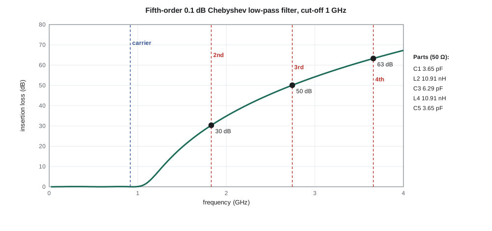
Thirty decibels at the second harmonic is not enough, as lesson 6 will show, and real parts make it worse: the 10.91 nH inductors have SRFs not far above 3 GHz, and parasitic capacitance across them lets the third and fourth harmonics leak past. Priya has three ways to improve the filter: raise the order, which adds loss at 915 MHz; convert it to an elliptic design with a transmission zero placed on the second harmonic; or add a separate trap, a series LC resonant at 1830 MHz connected from the line to ground. She chooses the trap for now, because it can be tuned on the bench, and keeps the elliptic design in reserve.

Distributed and acoustic filters

Above a few gigahertz, lumped parts give way to distributed filters made of coupled transmission-line resonators: edge-coupled, hairpin and interdigital filters, or stepped-impedance low-pass filters that alternate high- and low-impedance line sections in place of inductors and capacitors. They are cheap, because they are part of the board, but large and sensitive to the board's dielectric constant, and they suffer from spurious passbands at multiples of the design frequency. At 2.4 GHz a hairpin filter is a few centimetres long; at 915 MHz it would be impractically large.

Acoustic filters solve the size problem by converting the electrical signal into an acoustic wave, which travels about 100 000 times more slowly than an electromagnetic wave, so that resonators a wavelength long are only micrometres in size. Surface acoustic wave (SAW) filters use interdigitated electrodes on a piezoelectric crystal to launch and receive waves along the surface. Bulk acoustic wave (BAW) filters use thin piezoelectric films between electrodes and work well to higher frequencies. Both give steep skirts and high rejection in packages of 1 to 3 mm, with insertion losses of 1 to 3 dB, and they are why every phone can contain dozens of band filters. Their weaknesses are limited power handling, a frequency drift with temperature of tens of parts per million per kelvin for SAW, and sensitivity to electrostatic discharge.

Amara's SAW filter for the cabinet receiver has 1.5 dB of loss across 902–928 MHz and a data-sheet rejection of more than 40 dB below 880 MHz and above 960 MHz. Its rejection close to the band edges is much smaller, and it cannot touch the paging transmitter at 930 MHz. Leo measures it on the fixture of lesson 2 at −40, 25 and 85 °C to confirm that the passband still covers the band at the temperature extremes of a sun-heated cabinet.

Baluns and other passive parts

Many transceiver chips, including the sub-GHz chip in TLR-2, have differential radio-frequency ports: two pins carrying signals of opposite phase. A balun (balanced-to-unbalanced transformer) converts them to a single 50 Ω port. At 915 MHz baluns are built from discrete LC networks, often combined with the matching network, or bought as small ceramic parts; at higher frequencies they can be made from coupled lines. Directional couplers sample forward and reflected power for monitoring, and transmit/receive switches, usually solid-state, connect the antenna to the power amplifier or to the receiver. Each of these adds a little loss, which the cascade calculations of lesson 1 must include.