The Smith chart and impedance matching networks

The sub-GHz transceiver that Amara has chosen for TLR-2 has a receive input that is not 50 Ω. Its data sheet gives the input impedance at 915 MHz as 25 − j60 Ω, a small resistance in series with a capacitance, typical of the gate of an integrated LNA with its pad and bond wire. Connected directly to a 50 Ω line it would reflect most of the incoming signal: |Γ| is about 0.62, a mismatch loss of 2.4 dB and a large noise penalty. Its 20 dBm power amplifier output wants to see about 12 Ω, not 50 Ω, to deliver its rated power from its supply voltage. Both need matching networks, small circuits of inductors, capacitors or transmission lines that transform one impedance into another with as little loss as possible.

ELE-360 introduced the Smith chart and used one stub and one quarter-wave transformer on the TLR-1 antenna feed. This lesson goes deeper: it develops the Smith chart as a design tool for lumped networks, designs L, Pi and T networks, relates their quality factor to bandwidth and harmonic rejection, and compares lumped and distributed matching. By the end Priya can draw a match on the chart and calculate its parts in a few minutes, and check the result with a short program.

The Smith chart as a design tool

The Smith chart is a plot of the complex reflection coefficient Γ inside the unit circle, overlaid with circles of constant normalized resistance r and arcs of constant normalized reactance x, where z = Z/Z₀ = r + jx. The centre is z = 1, a perfect match; the left edge is a short and the right edge an open. Because Γ = (z − 1)/(z + 1) maps the right half of the impedance plane into the unit circle, every passive impedance, however extreme, has a place on the chart.

The chart's power as a design tool comes from how simple elements move an impedance across it. Adding a series reactance changes x but not r, so the impedance moves along a constant-resistance circle: clockwise (upward) for a series inductor and anticlockwise (downward) for a series capacitor. Adding a shunt susceptance changes the admittance y = g + jb but not its conductance g, so the point moves along a constant-conductance circle, which is a constant-resistance circle reflected through the centre. A shunt capacitor moves the point clockwise along that circle and a shunt inductor anticlockwise. A length of lossless 50 Ω line rotates the point clockwise around the centre, by twice the electrical length. With these three moves, a designer can see on the chart every possible way of reaching the centre from a given load.

Charts printed with both impedance and admittance grids, called ZY charts, make this easy by hand. In practice engineers use the chart in software, but the geometric picture remains the best way to understand why a match works, how wide it will be and what happens when a component value drifts.

L networks

The simplest lumped match uses two reactive elements in an L: one in series and one in shunt. For a purely resistive load R_L and source R_S, the L network has a single quality factor fixed by the ratio of the two resistances, and the element nearest the smaller resistance is in series.

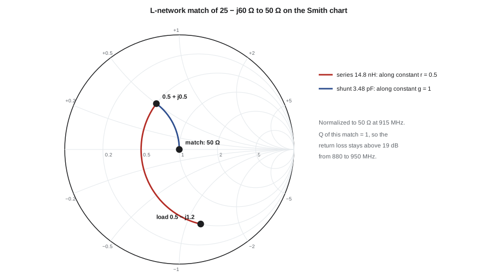
A complex load is handled by first absorbing its reactance: the series element is chosen to cancel the load's reactance and add the required X_s at the same time. For the transceiver input, R_L = 25 Ω and R_S = 50 Ω, so Q = 1. The series element next to the load must give a total reactance of +25 Ω, so it adds +85 Ω to cancel the −60 Ω of the load; the shunt element at the 50 Ω side must supply a susceptance of 0.02 S. There are always two solutions, one with the shunt element capacitive and one inductive, which the program below finds.

import math, cmath

f = 915e6; w = 2*math.pi*f; Z0 = 50.0
def comp(X):
    """Reactance in ohms -> part value at f."""
    return f"L = {X/w*1e9:5.2f} nH" if X > 0 else f"C = {-1/(w*X)*1e12:5.2f} pF"

# 1. L-network from 50 ohms to the transceiver input ZL = 25 - j60 ohms
ZL = 25 - 60j
RL, XL = ZL.real, ZL.imag
# load resistance below 50: series element next to the load, shunt element at the 50-ohm side
Q = math.sqrt(Z0/RL - 1)
for sgn in (+1, -1):
    Xs = sgn*Q*RL - XL           # series reactance added to the load
    Bp = sgn*Q/Z0                # shunt susceptance at the source side (its sign follows Xs)
    Xp = -1/Bp
    Zin = 1/(1/(ZL + 1j*Xs) + 1/(1j*Xp))
    print(f"solution {'+' if sgn > 0 else '-'}: series {comp(Xs)}, shunt {comp(Xp)}, Zin = {Zin.real:5.1f} {Zin.imag:+5.1f}j ohm, Q = {Q:.2f}")

# 2. Bandwidth of the first solution: sweep 860-970 MHz with fixed part values
Xs0 = Q*RL - XL; Xp0 = -1/(Q/Z0)
Ls = Xs0/w; Cp = 1/(w*-Xp0) if Xp0 < 0 else None; Lp = Xp0/w if Xp0 > 0 else None
for fm in (880e6, 902e6, 915e6, 928e6, 950e6):
    wm = 2*math.pi*fm
    zl = 25 + 1j*(-60*w/wm)                   # load reactance treated as a capacitor
    xs = wm*Ls if Xs0 > 0 else -1/(wm*(-1/(w*Xs0)))
    xp = -1/(wm*Cp) if Cp else wm*Lp
    zin = 1/(1/(zl + 1j*xs) + 1/(1j*xp))
    g = abs((zin - Z0)/(zin + Z0))
    rl = -20*math.log10(g) if g > 1e-4 else float('inf')
    print(f"   {fm/1e6:5.0f} MHz  |Gamma| {g:.3f}  return loss {rl:5.1f} dB")

# 3. Pi network for the 20 dBm PA: 12 ohm load line to 50 ohm, loaded Q chosen as 3
Rp, Rl, Qp = 12.0, 50.0, 3.0
Rv = Rl/(1 + Qp**2)                # virtual resistance in the middle of the Pi, set by Q at the 50-ohm end
Q1 = math.sqrt(Rp/Rv - 1); Q2 = math.sqrt(Rl/Rv - 1)
C1 = Q1/(w*Rp); C2 = Q2/(w*Rl); Lser = (Q1 + Q2)*Rv/w
print(f"Pi match 12 -> 50 ohm: Rv {Rv:.2f} ohm, C1 {C1*1e12:.1f} pF, L {Lser*1e9:.2f} nH, C2 {C2*1e12:.1f} pF (Q1 {Q1:.2f}, Q2 {Q2:.2f})")
print(f"simple L match 12 -> 50 would have Q = {math.sqrt(50/12 - 1):.2f}")

# 4. Single shunt short-circuited stub on 50-ohm line to match ZL
yl = Z0/ZL
best = None
for k in range(1, 5000):
    d = k/10000.0                      # distance in wavelengths
    t = math.tan(2*math.pi*d)
    y = (yl + 1j*t)/(1 + 1j*yl*t)
    if abs(y.real - 1) < 0.002:
        best = (d, y); break
d, y = best
b = -y.imag                            # stub must add this susceptance
ls = math.atan(1/(-b))/(2*math.pi) % 0.5  # short stub: y = -j cot(beta l), so cot(beta l) = -b
print(f"stub: d = {d:.4f} lambda, stub length {ls:.4f} lambda (y at stub point {y.real:.3f}{y.imag:+.3f}j)")

solution +: series L = 14.78 nH, shunt C =  3.48 pF, Zin =  50.0  +0.0j ohm, Q = 1.00
solution -: series L =  6.09 nH, shunt L =  8.70 nH, Zin =  50.0  +0.0j ohm, Q = 1.00
     880 MHz  |Gamma| 0.111  return loss  19.1 dB
     902 MHz  |Gamma| 0.042  return loss  27.6 dB
     915 MHz  |Gamma| 0.000  return loss   inf dB
     928 MHz  |Gamma| 0.042  return loss  27.6 dB
     950 MHz  |Gamma| 0.113  return loss  19.0 dB
Pi match 12 -> 50 ohm: Rv 5.00 ohm, C1 17.2 pF, L 3.64 nH, C2 10.4 pF (Q1 1.18, Q2 3.00)
simple L match 12 -> 50 would have Q = 1.78
stub: d = 0.0814 lambda, stub length 0.0793 lambda (y at stub point 0.999+1.838j)

The first solution uses a series 14.8 nH inductor and a shunt 3.48 pF capacitor; the second uses a series 6.09 nH inductor and a shunt 8.70 nH inductor. Both give a perfect match at 915 MHz. Priya prefers the first. The shunt capacitor at the antenna side gives a low-pass response that adds a little rejection of the harmonics and of signals above the band, and a series inductor with a shunt capacitor is easier to tune on the bench by changing the capacitor. The second solution's shunt inductor provides a DC path to ground, which is useful if the input needs a DC return, and a high-pass response that rejects low-frequency signals; it would be the choice if the 460 MHz land-mobile transmitters measured in lesson 1 were the bigger worry.

Because Q = 1, the match is broad: the program shows a return loss above 27 dB across 902–928 MHz and above 19 dB from 880 to 950 MHz, even though the load reactance itself changes with frequency. A low-Q match is forgiving of component tolerance too, which matters with ±0.1 pF capacitors and ±2 % inductors.

Quality factor and bandwidth

Matching networks are resonant circuits, and their quality factor sets their bandwidth. For a simple L match, the loaded Q of the network is roughly the Q computed above, and the fractional bandwidth over which the match is good is roughly 1/Q. Matching 50 Ω to 25 Ω (Q = 1) is broadband; matching 50 Ω to 2 Ω, as the output of a high-power transistor sometimes requires, gives Q = 4.9 and a bandwidth of only about 20 % of the centre frequency. Large impedance ratios therefore call for several stages, each with a modest ratio. A two-section L match from 2 Ω to 50 Ω through 10 Ω has two sections with Q = 2 each and a much wider bandwidth than one section with Q = 4.9.

The theoretical limit is the Bode–Fano criterion, which says that a load containing reactance cannot be matched perfectly over a wide band: the integral of the return loss over frequency is bounded by the load's own Q. A small antenna, with its large stored energy, can therefore only be matched over a narrow band no matter how clever the network, a point lesson 8 returns to through the Chu limit.

Pi and T networks

An L network has no free parameter: its Q is fixed by the resistance ratio. Adding a third element gives one degree of freedom. A Pi network, two shunt elements with a series element between them, can be seen as two L networks back to back, each transforming to an imaginary virtual resistance R_v in the middle that is lower than both end resistances. A T network does the same with a virtual resistance higher than both. The designer chooses the loaded Q, and with it R_v.

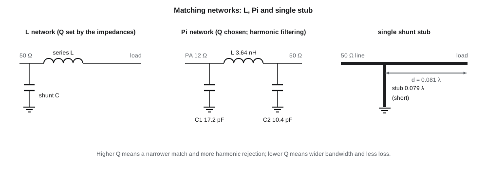
The Pi network is the classic output match for power amplifiers because its shunt capacitors absorb the transistor's output capacitance at one end and form a low-pass filter that attenuates harmonics. For the TLR-2 power amplifier's 12 Ω load line, Priya chooses Q = 3 at the 50 Ω end. The program gives R_v = 5 Ω, C₁ = 17.2 pF on the transistor side, a series 3.64 nH inductor, and C₂ = 10.4 pF at the 50 Ω side. A plain L match from 12 Ω to 50 Ω would have Q = 1.78 and less harmonic rejection; lesson 6 calculates how much the Pi network's higher Q contributes to the harmonic filtering.

Distributed matching

At 915 MHz, lumped parts work well: inductors and capacitors are much smaller than a wavelength and their parasitics, covered in lesson 4, are manageable. At higher frequencies, and for low-loss or high-power matching, transmission-line elements become attractive. ELE-360 used two: the single stub and the quarter-wave transformer. The single shunt stub places a short- or open-circuited line at a distance d from the load where the admittance has a real part equal to 1/Z₀, then cancels the remaining susceptance with the stub. For the transceiver input, the program finds d = 0.081 λ and a short-circuited stub 0.079 λ long. On the TLR-2 board, where the guided wavelength in 50 Ω microstrip is about 179 mm at 915 MHz, those are 14.6 mm and 14.2 mm: possible, but longer than the lumped network, which fits in 2 × 3 mm.

Distributed matching wins at 2.4 GHz and above, where lines are shorter and lumped parts have lower self-resonant frequencies. The BLE antenna match in lesson 8 combines a short length of line with lumped parts. Amara's rule of thumb for the team is to use lumped parts below about 2 GHz on TLR-2, and to treat every line longer than a twentieth of a wavelength as a circuit element that must appear in the simulation.

Matching for noise, power and linearity

A matching network is not always designed for maximum power transfer. The input of a low-noise amplifier is matched for minimum noise figure, which usually needs a source impedance different from the conjugate of the transistor's input impedance; lesson 5 shows how to compromise between noise and return loss. The output of a power amplifier is matched to the load line that gives the required output power and efficiency, which is far from a conjugate match; lesson 6 explains why. In both cases the matching network still transforms 50 Ω to a chosen impedance, and the Smith chart techniques of this lesson apply unchanged; only the target point is different.

Losses in the matching network deserve attention. A network with loaded Q_L built from inductors with unloaded Q_U loses roughly Q_L/Q_U of the power, expressed as a fraction. With Q_L = 3 and 0402 inductors of Q_U ≈ 35, the Pi network dissipates roughly 8 % of the power amplifier's output, about 0.4 dB; in an LNA, the same loss in front of the transistor adds directly to the noise figure. Low-Q matches with high-Q parts are therefore preferred wherever bandwidth and harmonic rejection allow.