
ELE-360 · Lesson 7 of 12 · 25 min
Uniform plane waves
Far from the TLR-1 antenna, the wave it launches looks locally like the simplest solution of Maxwell's equations: a uniform plane wave, in which the electric and magnetic fields are perpendicular to each other and to the direction of travel and are the same everywhere on each plane perpendicular to that direction. Real waves spread out from their sources, but a few wavelengths from an antenna the spreading is so gradual that over any small region the wave is plane. Almost everything engineers need to know about propagation, from how fast a signal travels and how much it weakens in concrete to how deep currents penetrate into a metal enclosure and how much power a person standing near an antenna absorbs, can be learned from plane waves. This lesson develops them in lossless and lossy media, introduces the Poynting vector for power flow and describes polarization.
The plane wave in a lossless medium
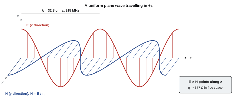
Take the phasor wave equation of lesson 6 in a source-free lossless medium and look for a field that depends only on z. Let E point along x. The equation reduces to d²E_x/dz² + β²E_x = 0, with β = ω√(με). Its solutions are E_x = E⁺e^{−jβz} + E⁻e^{+jβz}: a wave travelling in +z and one travelling in −z. In the time domain the forward wave is E⁺ cos(ωt − βz), a cosine pattern sliding along z at the phase velocity v_p = ω/β = 1/√(με). The wavelength is λ = 2π/β = v_p/f. The phase constant β, in radians per metre, is also called the wavenumber k.
Faraday's law then fixes the magnetic field: H points along y, in phase with E, with magnitude E/η. The ratio η = √(μ/ε) is the intrinsic impedance of the medium, measured in ohms. In free space η₀ = √(μ₀/ε₀) ≈ 376.7 Ω, often rounded to 377 Ω or written 120π. In a dielectric with ε_r, η = η₀/√ε_r, so in polyethylene it is about 251 Ω and in FR-4 about 180 Ω. The directions of E, H and propagation form a right-handed set: E × H points in the direction of travel. A wave travelling in −z has its H reversed relative to E. These relations, E and H perpendicular, in phase and in the ratio η, are the plane-wave rules you will use constantly.
Worked problem
The TLR-1 wave in free space
The TLR-1 operates at 915 MHz. Find the wavelength and phase constant in free space and in polyethylene (ε_r = 2.25), and the magnetic field that accompanies an electric field of 1 V/m rms in free space.
Show solution
- \[\lambda_0 = \frac{c}{f} = \frac{2.998\times10^8}{915\times10^6} = 0.328\ \text{m} \qquad \beta_0 = \frac{2\pi}{\lambda_0} = 19.2\ \text{rad/m}\]
- \[\lambda_{\text{PE}} = \frac{\lambda_0}{\sqrt{2.25}} = 0.218\ \text{m} \qquad \beta_{\text{PE}} = 28.8\ \text{rad/m}\]
- \[H = \frac{E}{\eta_0} = \frac{1}{376.7} = 2.65\ \text{mA/m rms}\]
Answer: A wavelength of 32.8 cm in air and 21.8 cm in the cable dielectric, and 2.65 mA/m of magnetic field per volt per metre of electric field. The quarter-wave whip of lesson 12 is about 8 cm long because of this wavelength.
Power flow: the Poynting vector
Electromagnetic waves carry energy. Poynting's theorem, derived by combining Maxwell's curl equations, shows that the rate at which energy flows out of a closed surface equals the rate of decrease of stored field energy inside minus the power dissipated in it. The power flow per unit area is the Poynting vector S = E × H, in watts per square metre. For sinusoidal fields, the time-average Poynting vector is ½Re(E × H*) with peak phasors, or Re(E × H*) with rms phasors. For a plane wave in a lossless medium this is |E|²/η, using rms values. Power density is what radiation exposure limits restrict and what a receiving antenna collects, so lessons 11 and 12 use it constantly.
Poynting's theorem has a surprising consequence even in circuits. In a coaxial cable carrying DC power, the energy does not flow inside the copper; it flows through the dielectric between the conductors, carried by the radial electric field and the circling magnetic field, whose cross product points along the cable. The copper guides the energy and dissipates a little of it as heat, but the energy itself travels in the fields. The same is true on a printed-circuit board: the signal energy travels in the dielectric between a trace and its ground plane, which is why lesson 11 cares so much about what lies under a trace.
Waves in lossy media
In a conducting medium, ∇×H = (σ + jωε)E, and the wave equation acquires a complex propagation constant γ = α + jβ = √(jωμ(σ + jωε)). The wave becomes E⁺e^{−αz}e^{−jβz}: it still oscillates with phase constant β but its amplitude decays by the attenuation constant α, in nepers per metre. Multiply α by 8.686 to get decibels per metre. The intrinsic impedance becomes complex, η = √(jωμ/(σ + jωε)), so H lags E in phase. The depth at which the amplitude falls to 1/e, about 37 percent, is 1/α.
Two limits make γ easy. In a low-loss dielectric, σ ≪ ωε, the attenuation is α ≈ (σ/2)√(μ/ε) = (σ/2)η and β is almost unchanged. If the loss is described by a loss tangent instead, α ≈ (β tan δ)/2. In a good conductor, σ ≫ ωε, α and β become equal, both √(πfμσ), and the wave decays by a factor of e in a distance δ = 1/√(πfμσ), the skin depth. At radio frequencies δ is tiny in metals: about 2.2 µm in copper at 915 MHz. Currents on metal surfaces flow only in this thin layer, which is why radio-frequency conductors behave as though their resistance per square were the surface resistance R_s = 1/(σδ), and why silver plating a few micrometres thick improves a connector even though the bulk metal is brass.
| Medium at 915 MHz | σ/(ωε) | Attenuation | Behaviour |
|---|---|---|---|
| Air | ≈ 0 | ≈ 0 | Lossless |
| Polyethylene cable dielectric | ≈ 0.0002 (tan δ) | very small | Low-loss dielectric |
| Concrete | about 0.05–0.15 | about 4–20 dB/m | Lossy dielectric; varies with moisture |
| Wet soil | about 0.05–0.2 | about 10–30 dB/m | Lossy dielectric |
| Seawater | about 1 | hundreds of dB/m | Neither: strongly lossy |
| Copper | ≈ 10⁹ | skin depth 2.2 µm | Good conductor |
Skin depth and shielding
Skin depth decides whether a metal enclosure shields. A wave striking a conducting wall is mostly reflected, as lesson 8 explains, and what enters decays by about 8.7 dB per skin depth. A sheet several skin depths thick therefore adds tens of decibels of absorption loss on top of the reflection loss. At 915 MHz, the 1.5 mm aluminium of the TLR-1 enclosure is hundreds of skin depths thick, so the metal itself is effectively opaque; in practice the shielding is limited by seams, gaps and openings, which lesson 8 also addresses. At the loop detector's 71 kHz, the skin depth in aluminium is about 0.3 mm, so the same enclosure still absorbs well. At 60 Hz, the skin depth in aluminium is about 11 mm and the enclosure barely affects power-frequency magnetic fields, which is why hum from a nearby luminaire cable must be fought with twisted pairs and balanced inputs rather than with thin metal.
Worked problem
Skin depth in the enclosure
The TLR-1 enclosure is 1.5 mm aluminium (σ = 3.5 × 10⁷ S/m). Find the skin depth and the absorption loss through the wall at 915 MHz, and the skin depth at 60 Hz.
Show solution
- \[\delta_{915} = \frac{1}{\sqrt{\pi \times 915\times10^6 \times 4\pi\times10^{-7} \times 3.5\times10^7}} = 2.81\ \mu\text{m}\]
- \[A = 8.686\,\frac{t}{\delta} = 8.686 \times \frac{1.5\times10^{-3}}{2.81\times10^{-6}} \approx 4600\ \text{dB}\]
- \[\delta_{60} = \delta_{915}\sqrt{\frac{915\times10^6}{60}} = 2.81\ \mu\text{m} \times 3905 = 11.0\ \text{mm}\]
Answer: The wall is about 530 skin depths thick at 915 MHz, so absorption through solid metal is astronomically large and irrelevant; leakage through openings dominates. At 60 Hz the wall is only 0.14 skin depths thick and provides almost no magnetic shielding.
import math, cmath
eps0, mu0, c = 8.854e-12, 4e-7 * math.pi, 2.998e8
eta0 = math.sqrt(mu0 / eps0)
print(f"free space: eta0 = {eta0:.1f} ohm, lambda at 915 MHz = {c / 915e6 * 100:.1f} cm")
# 1. Skin depth at three frequencies and surface resistance at 915 MHz
print("metal              60 Hz       71.2 kHz     915 MHz     Rs at 915 MHz")
for name, sig, mur in (("copper", 5.8e7, 1), ("aluminum", 3.5e7, 1), ("stainless (304)", 1.4e6, 1), ("mild steel", 6e6, 200)):
    ds = [1 / math.sqrt(math.pi * f * mu0 * mur * sig) for f in (60, 71.2e3, 915e6)]
    print(f"{name:16s} {ds[0]*1e3:8.3f} mm {ds[1]*1e3:8.4f} mm {ds[2]*1e6:8.3f} um   {1 / (sig * ds[2]) * 1e3:6.2f} mohm")
# 2. Exact propagation constant at 915 MHz (effective conductivity includes dielectric loss)
w = 2 * math.pi * 915e6
print("medium            alpha (dB/m)   lambda (cm)   |eta| (ohm)")
for name, er, sig in (("dry concrete", 5, 5e-3), ("typical concrete", 6, 3e-2), ("wet soil", 15, 5e-2), ("fresh water", 80, 0.2), ("seawater", 81, 4.0)):
    gam = cmath.sqrt(1j * w * mu0 * (sig + 1j * w * er * eps0))
    eta = cmath.sqrt(1j * w * mu0 / (sig + 1j * w * er * eps0))
    print(f"{name:16s} {gam.real * 8.686:10.2f}     {2 * math.pi / gam.imag * 100:9.2f}     {abs(eta):9.1f}")
# 3. Power density near the TLR-1 cabinet antenna and the general-public reference levels
eirp = 10 ** ((20 + 6 - 2) / 10) / 1000          # 20 dBm, 6 dBi panel, 2 dB cable loss -> W
for r in (0.2, 0.5, 2.0):
    S = eirp / (4 * math.pi * r * r)
    print(f"r = {r:3.1f} m: S = {S:7.4f} W/m^2, E = {math.sqrt(S * eta0):5.2f} V/m rms")
f = 915
print(f"reference levels at {f} MHz: Safety Code 6 {0.02619 * f**0.6834:.2f} W/m^2, FCC general population {f / 1500 * 10:.2f} W/m^2")free space: eta0 = 376.7 ohm, lambda at 915 MHz = 32.8 cm metal 60 Hz 71.2 kHz 915 MHz Rs at 915 MHz copper 8.532 mm 0.2477 mm 2.185 um 7.89 mohm aluminum 10.983 mm 0.3188 mm 2.812 um 10.16 mohm stainless (304) 54.914 mm 1.5941 mm 14.062 um 50.80 mohm mild steel 1.876 mm 0.0544 mm 0.480 um 347.00 mohm medium alpha (dB/m) lambda (cm) |eta| (ohm) dry concrete 3.66 14.65 168.5 typical concrete 20.01 13.36 153.4 wet soil 21.11 8.46 97.2 fresh water 36.57 3.66 42.1 seawater 664.76 3.33 35.5 r = 0.2 m: S = 0.4997 W/m^2, E = 13.72 V/m rms r = 0.5 m: S = 0.0800 W/m^2, E = 5.49 V/m rms r = 2.0 m: S = 0.0050 W/m^2, E = 1.37 V/m rms reference levels at 915 MHz: Safety Code 6 2.77 W/m^2, FCC general population 6.10 W/m^2
The skin-depth table confirms the worked example and adds two lessons. Stainless steel, a poor conductor, has a skin depth about six times that of copper and a surface resistance about six times higher, which is why stainless hardware near an antenna is lossy. Mild steel has a much smaller skin depth than its conductivity alone would suggest, because its permeability concentrates the current further; its high surface resistance is why a steel pole or a rebar cage absorbs some radio energy. The propagation table uses effective conductivities that include the dielectric relaxation loss at 915 MHz, so they are much larger than the direct-current values in lesson 6. Concrete attenuates the TLR-1 signal by several to around 20 dB per metre depending on its moisture, wet soil similarly, fresh water more, and seawater stops it within centimetres. Those numbers explain why the radio works across an intersection but not from inside a buried vault.
Exposure to radio-frequency fields
Health Canada's Safety Code 6 sets reference levels for human exposure, and ISED's RSS-102 applies them to radio equipment. For the general public between 300 MHz and 6 GHz, the reference level for power density rises with frequency, 0.02619 f^0.6834 W/m² with f in MHz, which is about 2.8 W/m² at 915 MHz, averaged over 6 minutes. The power density near the TLR-1 cabinet antenna, with 24 dBm of effective isotropic radiated power from a 20 dBm transmitter, a 6 dBi antenna and 2 dB of cable loss, is about 0.5 W/m² at 20 cm and 0.08 W/m² at 0.5 m, and the antenna sits on a mast arm several metres above the sidewalk. The far-field formula overestimates the density very close to an antenna, and the regulator's evaluation methods take that into account, but even this simple estimate shows a large margin. The US limit, for comparison, is about 6.1 W/m² at the same frequency.
Polarization
The polarization of a wave describes the path traced by the tip of its electric field vector at a fixed point. If E always points along one line, the wave is linearly polarized; a vertical whip antenna radiates vertical linear polarization. If E has two perpendicular components of equal amplitude 90° out of phase, the tip traces a circle and the wave is circularly polarized, right-hand or left-hand depending on the direction of rotation relative to the direction of travel. In general the components have unequal amplitudes or an arbitrary phase and the tip traces an ellipse. Satellite navigation signals use circular polarization so that the receiver's orientation and the rotation of polarization by the ionosphere do not matter.
Polarization matters because a receiving antenna responds only to the field component that matches its own polarization. A vertical receiving whip picks up a vertically polarized wave fully and a horizontally polarized wave hardly at all; the polarization loss factor is cos²ψ, where ψ is the angle between the polarizations, so a 45° mismatch costs 3 dB and a 90° mismatch, in theory, everything. A linearly polarized antenna receiving a circularly polarized wave loses 3 dB whatever its orientation. For the TLR-1, Amara specifies vertical polarization at both ends of every link. Reflections from building walls and vehicles partly rotate the polarization, which lesson 8 explains, so in a cluttered intersection the polarization mismatch loss is a few decibels rather than the large values of a clean test range.
Common mistakes
MistakeForgetting that H in a plane wave is E divided by η, not by 377 Ω in every medium.
InsteadUse η = η₀/√ε_r in dielectrics and the complex η in lossy media.
MistakeUsing the low-loss attenuation formula in a good conductor.
InsteadCheck σ/(ωε) first; in good conductors α = β = 1/δ.
MistakeThinking thicker metal improves enclosure shielding at radio frequencies.
InsteadAny practical sheet is many skin depths thick; seams and openings limit shielding.
MistakeUsing peak phasors in the rms power formula.
Instead⟨S⟩ = ½Re(E×H*) with peak values, Re(E×H*) with rms values.
Summary and key terms
- A uniform plane wave has E and H perpendicular, in phase and in the ratio η; E × H points along propagation.
- β = ω√(με), v_p = 1/√(με) and λ = 2π/β; in free space η₀ ≈ 377 Ω.
- The Poynting vector E × H gives power flow per unit area; for a plane wave ⟨S⟩ = E²_rms/η.
- In lossy media the wave decays as e^{−αz}; low-loss dielectrics and good conductors have simple approximations.
- Skin depth δ = 1/√(πfμσ) is micrometres in metals at radio frequencies; surface resistance is 1/(σδ).
- Polarization describes the path of the E vector; mismatched polarizations lose cos²ψ of the power.
- Uniform plane wave
- A wave whose fields are uniform over planes perpendicular to the direction of travel.
- Phase constant
- β, the rate of phase change with distance, in radians per metre.
- Intrinsic impedance
- η, the ratio of E to H in a plane wave in a medium.
- Poynting vector
- S = E × H, the power flow per unit area.
- Attenuation constant
- α, the rate of amplitude decay with distance, in nepers per metre.
- Skin depth
- The depth at which a field or current in a conductor falls to 1/e of its surface value.
- Surface resistance
- R_s = 1/(σδ), the resistance per square of a conductor at high frequency.
- Polarization
- The orientation and path traced by a wave's electric field vector at a fixed point.
Practice problems
Work each problem on paper first, then reveal the answer to check.
A plane wave in air has E = 5 V/m rms. Find H and the power density.
Show answer
13.3 mA/m; 0.0664 W/m².
Find the wavelength at 2.45 GHz in free space and in a medium of ε_r = 4.
Show answer
12.2 cm; 6.1 cm.
Find the skin depth of copper at 10 MHz.
Show answer
20.9 µm.
A dielectric has ε_r = 4.4 and tan δ = 0.02 at 915 MHz. Estimate α in dB/m.
Show answer
β = 40.3 rad/m; α ≈ βtanδ/2 = 0.403 Np/m = 3.5 dB/m.
A wave of 1 W/m² is incident on a vertical antenna with polarization tilted 30° from vertical. What fraction of the power is matched?
Show answer
cos²30° = 0.75, a loss of 1.25 dB.
An isotropic source radiates 0.1 W. What is the power density 1 m away?
Show answer
0.1/(4π) = 7.96 mW/m².
Lesson quiz · 5 questions
Score 60% or more to complete this lesson.
Create a free account to save your progress, take quizzes and earn a certificate.