
ELE-360 · Lesson 6 of 12 · 25 min
Maxwell's equations
By the 1860s, the laws of Coulomb, Gauss, Ampère and Faraday were well established, each tested in the laboratory. James Clerk Maxwell set out to write them as one consistent set and found that they were not consistent. Ampère's law, as written in lesson 4, contradicts the conservation of charge whenever charge is piling up somewhere, as it does on a capacitor plate. Maxwell repaired the law by adding a term he called the displacement current. The repaired equations predicted something nobody had looked for: electric and magnetic fields that sustain each other and travel through empty space at a speed that, when he calculated it from the measured values of ε₀ and μ₀, matched the measured speed of light. Light was an electromagnetic wave. Two decades later Heinrich Hertz generated and detected such waves at radio frequencies, and every radio since, the TLR-1 included, is an application of that discovery.
This lesson assembles the four equations, explains the displacement current and the continuity of charge, writes the equations in the phasor form used for sinusoidal steady state, and shows how they predict waves. It also gives two practical tools Amara uses every week: a test for whether a material behaves as a conductor or a dielectric at a given frequency, and a test for whether a structure is small enough to treat as a lumped circuit.
Conservation of charge
Charge cannot be created or destroyed, so if current flows out of a closed region, the charge inside must fall. Written for a closed surface, the net outward current equals the rate of decrease of enclosed charge. Applying the divergence theorem gives the continuity equation at a point: ∇·J = −∂ρ_v/∂t. For steady currents, ∂ρ_v/∂t = 0 and the divergence of J is zero, which is Kirchhoff's current law at a point. When charge accumulates, as on a capacitor plate during charging, J has a divergence equal to the rate of accumulation.
The displacement current
Take the divergence of Ampère's law as written in lesson 4, ∇×H = J. The divergence of any curl is zero, so this requires ∇·J = 0 always, which contradicts the continuity equation whenever charge is changing. A concrete picture makes the problem vivid. A capacitor is charging, with current I in the wire. Draw a circle round the wire and apply Ampère's law using a flat surface that the wire pierces: the enclosed current is I. Now keep the same circle but bulge the surface out so that it passes between the capacitor plates instead. No conduction current crosses it, so the enclosed current is zero. The circulation of H round one circle cannot have two values.
Maxwell's fix was to add ∂D/∂t to the current density. Between the plates the charge on the plates is growing, so D = ρ_S between them is growing, and the flux of ∂D/∂t through the bulging surface equals exactly the conduction current I in the wire. The modified law gives the same circulation for both surfaces. Taking its divergence now gives ∇·J + ∂(∇·D)/∂t = ∇·J + ∂ρ_v/∂t = 0, which is the continuity equation. The added term is called the displacement current density. It is not a flow of charge, but it produces a magnetic field exactly as a conduction current does, and that is what lets a changing electric field create a magnetic field even in empty space.
Worked problem
Displacement current in a capacitor
A 100 pF capacitor with plates 20 mm × 20 mm carries a 1 V, 1 MHz sinusoidal voltage. Find the peak current in its leads and the peak displacement current density between its plates.
Show solution
- \[I = \omega C V = 2\pi \times 10^6 \times 100\times10^{-12} \times 1 = 0.628\ \text{mA}\]
- Between the plates, D = ρ_S = Q/A, so ∂D/∂t = (dQ/dt)/A = I/A.
- \[J_d = \frac{0.628\times10^{-3}}{(0.020)^2} = 1.57\ \text{A/m}^2\]
Answer: The displacement current between the plates equals the conduction current in the leads, 0.628 mA peak, spread over the plate area. Ampère's law with Maxwell's term holds on every surface.
The four equations
With the displacement current in place, the four equations below, together with the constitutive relations and the Lorentz force, describe all classical electromagnetic phenomena. Read them as sentences. Faraday: a changing magnetic field makes the electric field curl. Ampère–Maxwell: currents and a changing electric field make the magnetic field curl. Gauss: charges are the sources of electric flux. Gauss for magnetism: there are no magnetic sources, so magnetic flux lines close. The integral forms state the same laws for loops and closed surfaces, and the theorems of lesson 1 convert between the two.
| Law | Differential form | Integral form | Meaning |
|---|---|---|---|
| Faraday | ∇×E = −∂B/∂t | ∮E·dl = −d/dt ∫B·dS | Changing B induces a circulating E |
| Ampère–Maxwell | ∇×H = J + ∂D/∂t | ∮H·dl = I + d/dt ∫D·dS | Current and changing D produce a circulating H |
| Gauss | ∇·D = ρ_v | ∮D·dS = Q_enc | Charge is the source of electric flux |
| Gauss (magnetic) | ∇·B = 0 | ∮B·dS = 0 | No magnetic charges; flux lines close |
The equations are linear in the fields when the materials are linear, which is why superposition works and why the frequency-domain methods of circuit theory carry over. They are local: each says something about fields at one point and the rate of change there, so effects propagate from point to point rather than acting instantaneously at a distance. And they are symmetric between E and H apart from the missing magnetic charge and current, a symmetry that makes the analysis of antennas in lesson 12 much shorter than it would otherwise be.
Boundary conditions, in general
Lessons 3 and 4 found boundary conditions for static fields. The same four conditions hold for time-varying fields, because they come from applying the integral forms to vanishingly thin loops and pillboxes, and the time-derivative terms vanish as the loop or box shrinks. Tangential E is continuous. Tangential H jumps by any surface current density J_S. Normal D jumps by the surface charge. Normal B is continuous. At a perfect conductor, where all fields inside vanish, the tangential E and normal B outside are zero, the normal D equals ρ_S and the tangential H equals the surface current. These conditions, applied to waves, explain reflection in lesson 8 and the guided modes of lesson 11.
Sinusoidal steady state: phasors
Most of electrical engineering works at a single frequency or in a narrow band around one. For fields that vary sinusoidally at angular frequency ω, we write each field as the real part of a complex phasor times e^{jωt}, exactly as in AC circuit analysis. Each time derivative becomes multiplication by jω, and Maxwell's equations become algebraic in time. In a linear conducting medium, the conduction and displacement currents combine: ∇×H = (σ + jωε)E. The ratio of the two parts, σ/(ωε), tells you which dominates. When it is much greater than 1, the material is a good conductor at that frequency; when much less than 1, it is a good dielectric, and σ/(ωε) is then its loss tangent.
Electrically small and electrically large
Circuit theory is Maxwell's equations simplified for structures much smaller than a wavelength. In such structures, the fields at every point respond to the sources essentially instantaneously, the time a change takes to cross the structure is negligible compared with a period, and the fields can be summarized by voltages and currents on the terminals. A common rule of thumb treats anything smaller than about a tenth of a wavelength as lumped. At 60 Hz the wavelength is 5000 km, so a whole city's wiring is lumped for most purposes. At the loop detector's 71 kHz the wavelength is over 4 km, so the loop and its 50 m lead-in are tiny and the circuit model of lessons 4 and 5 is excellent. At the TLR-1's 915 MHz, the wavelength is 32.8 cm, so anything longer than about 3 cm, including most of the radio's board traces and every cable, must be treated as a transmission line or an antenna.
Fast digital edges and electrostatic discharge are broadband. A pulse with a rise time t_r has significant spectral content up to roughly 0.35/t_r, so a discharge that rises in under a nanosecond reaches into the gigahertz range, with wavelengths of tens of centimetres down to a few centimetres. That is why a few centimetres of ground strap can have a significant inductive voltage across it during a discharge, and why the strap's length and routing matter as much as its resistance. The rule of thumb is crude, and lesson 9 will replace it with a better one, but it tells you immediately when the methods of this course are needed.
The wave equation
In a source-free, lossless region, take the curl of Faraday's law and substitute the Ampère–Maxwell law. Using the vector identity ∇×∇×E = ∇(∇·E) − ∇²E and Gauss's law with no charge, ∇·E = 0, you obtain the wave equation for E, and the same steps give one for H. Its solutions are disturbances that travel without changing shape at speed 1/√(με). In free space this is c = 1/√(μ₀ε₀) ≈ 2.998 × 10⁸ m/s. In a material with ε_r and μ_r = 1, the speed is c/√ε_r, so the TLR-1 signal travels at about two thirds of c in polyethylene coaxial cable and about half of c inside FR-4.
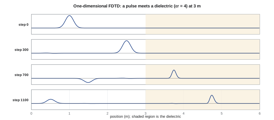
The wave equation can be solved numerically by stepping Maxwell's two curl equations forward in time on a grid, the finite-difference time-domain method. Electric and magnetic field samples sit at alternate grid points, offset by half a cell, and are updated in alternate half time steps, a scheme Kane Yee published in 1966. Each update uses only the neighbouring samples of the other field, which is Maxwell's locality made literal. The method is the basis of many commercial electromagnetic simulators. The Python block runs a one-dimensional version with a pulse crossing free space and entering a dielectric, and measures its speed in each region.
import math
eps0, mu0, c = 8.854e-12, 4e-7 * math.pi, 2.998e8
# 1. Conduction versus displacement current, sigma / (w eps), at three frequencies
mats = (("copper", 1, 5.8e7), ("seawater", 81, 4.0), ("wet soil", 15, 1e-2), ("damp concrete", 8, 1e-3))
print("material          60 Hz       71 kHz      915 MHz")
for name, er, sig in mats:
    print(f"{name:14s} " + "  ".join(f"{sig / (2 * math.pi * f * er * eps0):10.2e}" for f in (60, 71.2e3, 915e6)))
# 2. Electrical size: a structure is roughly lumped if it is shorter than lambda / 10
for f, what in ((60, "power line"), (71.2e3, "loop detector"), (915e6, "TLR-1 radio"), (5e9, "fast ESD edge")):
    lam = c / f
    print(f"{what:14s} f = {f:9.3g} Hz  lambda = {lam:9.3g} m  lumped below about {lam / 10:9.3g} m")
# 3. One-dimensional FDTD: a right-going Gaussian pulse in free space, then a dielectric (er = 4) from 3 m on
eta0 = math.sqrt(mu0 / eps0)
N, dz = 600, 0.01                  # 6 m in 1 cm cells
dt = dz / (2 * c)                  # Courant number 0.5
g = lambda z: math.exp(-((z - 1.0) / 0.15) ** 2)
Ex = [g(k * dz) for k in range(N)]                                  # pulse peak at 1 m
Hy = [-g((k + 0.5) * dz - c * dt / 2) / eta0 for k in range(N)]     # matching H makes it travel right
er = [1.0] * 300 + [4.0] * 300
peak = {}
for n in range(1300):
    for k in range(N - 1):
        Hy[k] += dt / (mu0 * dz) * (Ex[k + 1] - Ex[k])
    for k in range(1, N):
        Ex[k] += dt / (eps0 * er[k] * dz) * (Hy[k] - Hy[k - 1])
    for p in (150, 250, 350, 450):
        if abs(Ex[p]) > abs(peak.get(p, (0, 0.0))[1]): peak[p] = (n, Ex[p])
for a, b in ((150, 250), (350, 450)):
    v = (b - a) * dz / ((peak[b][0] - peak[a][0]) * dt)
print(f"pulse speed from {a * dz:.1f} m to {b * dz:.1f} m: {v / 1e8:.3f} x 10^8 m/s, peak field {peak[b][1]:.3f}")material 60 Hz 71 kHz 915 MHz copper 1.74e+16 1.46e+13 1.14e+09 seawater 1.48e+07 1.25e+04 9.70e-01 wet soil 2.00e+05 1.68e+02 1.31e-02 damp concrete 3.74e+04 3.16e+01 2.46e-03 power line f = 60 Hz lambda = 5e+06 m lumped below about 5e+05 m loop detector f = 7.12e+04 Hz lambda = 4.21e+03 m lumped below about 421 m TLR-1 radio f = 9.15e+08 Hz lambda = 0.328 m lumped below about 0.0328 m fast ESD edge f = 5e+09 Hz lambda = 0.06 m lumped below about 0.006 m pulse speed from 1.5 m to 2.5 m: 2.998 x 10^8 m/s, peak field 1.000 pulse speed from 3.5 m to 4.5 m: 1.495 x 10^8 m/s, peak field 0.664
The first table is the conductor-or-dielectric test. Copper is a conductor at every frequency here by a factor of at least a billion. Seawater is an excellent conductor at 60 Hz and at 71 kHz but drops to a ratio near 1 at 915 MHz, where it is a lossy dielectric; that is why submarines communicate at very low frequencies. Wet soil and damp concrete conduct at power and detector frequencies, which is why the loop's field induces small currents in the pavement, but both are fairly low-loss dielectrics at 915 MHz, so the radio wave partly reflects from the ground and partly penetrates it rather than being stopped in a thin skin. The numbers depend strongly on moisture and salt, so treat them as orders of magnitude. The second table is the electrical-size test from the text. The FDTD run launches a pulse of unit amplitude, measures 2.998 × 10⁸ m/s in free space and very nearly half that in the dielectric (the small shortfall is numerical dispersion of the grid), and finds a transmitted peak of about two thirds of the incident one, as the reflection formulas of lesson 8 will predict.
Electromagnetic potentials, briefly
Because ∇·B = 0, the magnetic field can always be written as the curl of a vector potential A, B = ∇×A. Faraday's law then lets E be written as −∇V − ∂A/∂t, extending the static E = −∇V. With a suitable choice of gauge, both potentials obey wave equations whose sources are the charge and current densities, and their solutions are the retarded potentials: the potential at a point and time is the sum of contributions from each source as it was a travel time R/v earlier. Retardation is the mathematical expression of the finite speed of light, and lesson 12 uses the retarded vector potential of a short current element to derive the fields of an antenna.
Common mistakes
MistakeDropping the displacement current at radio frequencies.
InsteadWithout ∂D/∂t there are no waves; it is essential whenever structures approach a tenth of a wavelength.
MistakeClassifying a material as a conductor or dielectric once and for all.
InsteadCompare σ with ωε at the frequency of interest; seawater and soil change category between kilohertz and gigahertz.
MistakeTreating a 10 cm trace at 915 MHz as a lumped wire.
InsteadIt is about a third of a wavelength in FR-4; analyse it as a transmission line.
MistakeForgetting that rise time sets bandwidth.
InsteadA nanosecond edge has content to hundreds of megahertz and beyond; wiring that is short at the clock rate may be long at the edge rate.
Summary and key terms
- Charge conservation gives the continuity equation ∇·J = −∂ρ_v/∂t.
- Maxwell added the displacement current ∂D/∂t to Ampère's law, making it consistent with charge conservation.
- The four equations with the constitutive relations describe all classical electromagnetic fields; their integral and differential forms are equivalent.
- Phasor form replaces ∂/∂t with jω; σ/(ωε) classifies a material as a conductor or a dielectric at each frequency.
- Structures smaller than about a tenth of a wavelength can be treated as lumped circuits; larger ones need field or transmission-line methods.
- Maxwell's equations imply wave equations with speed 1/√(με); FDTD solves them by stepping the curl equations in time.
- Continuity equation
- ∇·J = −∂ρ_v/∂t, the point form of conservation of charge.
- Displacement current
- The term ∂D/∂t in the Ampère–Maxwell law, which produces magnetic field like a conduction current.
- Constitutive relations
- D = εE, B = μH and J = σE, which describe how a material responds to fields.
- Phasor
- A complex amplitude representing a sinusoidal quantity at one frequency.
- Electrically small
- Much smaller than a wavelength, so lumped circuit models apply.
- Wave equation
- A second-order equation whose solutions are disturbances travelling at a fixed speed.
- FDTD
- Finite-difference time-domain: a numerical method that steps Maxwell's curl equations in time on a staggered grid.
- Retarded potential
- A potential computed from sources at the earlier time when their influence left them.
Practice problems
Work each problem on paper first, then reveal the answer to check.
A capacitor of 1 nF has 10 V at 100 kHz across it. What is the displacement current?
Show answer
ωCV = 6.28 mA peak.
Is wet soil (ε_r = 15, σ = 0.01 S/m) a conductor or a dielectric at 1 MHz?
Show answer
σ/(ωε) = 12, so it behaves as a moderately good conductor.
At what frequency does σ equal ωε for seawater (ε_r = 81, σ = 4 S/m)?
Show answer
σ/(2πε) = 888 MHz.
What is the speed of a signal in PTFE (ε_r = 2.1)?
Show answer
c/√2.1 = 2.07 × 10⁸ m/s.
Is a 4 cm trace lumped at 915 MHz on FR-4 (ε_eff ≈ 3.3)?
Show answer
λ = 32.8/√3.3 = 18 cm; λ/10 = 1.8 cm, so no.
Show that the surface integral of J + ∂D/∂t over any closed surface is zero.
Show answer
Its divergence is ∇·J + ∂ρ_v/∂t = 0 by continuity; the divergence theorem gives zero flux.
Lesson quiz · 5 questions
Score 60% or more to complete this lesson.
Create a free account to save your progress, take quizzes and earn a certificate.