
ELE-360 · Lesson 10 of 12 · 26 min
Transmission-line analysis and the Smith chart
Leo's first measurement of the prototype cabinet antenna on the network analyzer showed an impedance of about 70 + j15 Ω at 915 MHz, a VSWR of 1.52, just outside Amara's specification of 1.5. The antenna supplier's datasheet promised better, but that was measured on a large ground plane, not on a mast arm. Amara has three questions. What impedance will the radio see at the other end of the 12 m feeder? Can a small matching section at the antenna fix the mismatch, and over what bandwidth? And when a unit in the field reports poor performance a year later, how can a technician find out where along the cable the problem lies without taking it down? This lesson answers them with the input-impedance formula, matching sections, the Smith chart and time-domain reflectometry.
Input impedance of a terminated line
At a distance ℓ from a load Z_L, the voltage and current on a line are the sums of the forward and reflected waves, and their ratio is the impedance looking toward the load, Z_in. For a lossless line, Z_in depends on the load, the characteristic impedance and the electrical length βℓ. Equivalently, the reflection coefficient at distance ℓ is the load reflection rotated by −2βℓ: moving a quarter wavelength toward the generator rotates Γ by 180°, and a half wavelength by a full turn. Impedance therefore repeats every half wavelength, and a quarter wavelength inverts it.
Three special cases are worth memorizing. A short-circuited line has Z_in = jZ₀ tan βℓ: inductive for lengths under a quarter wavelength, an open circuit at exactly a quarter wavelength, then capacitive. An open-circuited line has Z_in = −jZ₀ cot βℓ, the reverse. These short sections of line, called stubs, act as inductors and capacitors at radio frequencies, and at microwave frequencies, where lumped components become unreliable, they are often the only practical reactances. Finally, a quarter-wave line transforms Z_L into Z₀²/Z_L. A quarter-wave short circuit therefore looks open, which is how a quarter-wave stub can support a centre conductor without affecting the signal, and a quarter-wave section with the right Z₀ can match two different resistances.
| Line section | Input impedance | Use |
|---|---|---|
| Matched, any length | Z₀ | Carries power without reflection |
| Short circuit, length ℓ < λ/4 | jZ₀ tan βℓ (inductive) | Inductor, shunt stub |
| Open circuit, length ℓ < λ/4 | −jZ₀ cot βℓ (capacitive) | Capacitor, shunt stub |
| Quarter wavelength, load Z_L | Z₀²/Z_L | Impedance transformer, impedance inverter |
| Half wavelength, load Z_L | Z_L | Repeats the load at a distance |
Worked problem
What the radio sees
The antenna presents 70 + j15 Ω to a 50 Ω lossless line. Find Γ_L and the input impedance at several distances from the load.
Show solution
- \[\Gamma_L = \frac{70 + j15 - 50}{70 + j15 + 50} = \frac{20 + j15}{120 + j15} = 0.207\angle 29.7^\circ \qquad \text{VSWR} = 1.52\]
- \[\ell = \lambda/8:\quad Z_{\text{in}} = 50\,\frac{70 + j15 + j50}{50 + j(70 + j15)} = 57.1 - j21.4\ \Omega\]
- \[\ell = \lambda/4:\quad Z_{\text{in}} = \frac{50^2}{70 + j15} = 34.1 - j7.3\ \Omega\]
- \[\ell = \lambda/2:\quad Z_{\text{in}} = 70 + j15\ \Omega\]
Answer: The magnitude of Γ, and so the VSWR, stays at 0.207 and 1.52 everywhere on a lossless line; only its phase rotates, carrying the impedance round a circle. Because the 12 m feeder is many wavelengths long, the impedance at the radio depends sensitively on its exact electrical length and on frequency, which is why mismatch should be fixed at the antenna, not at the radio.
The Smith chart
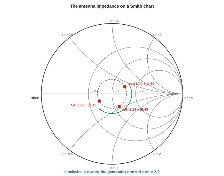
The Smith chart, devised by Phillip Smith in 1939, is a map of the complex Γ plane inside the unit circle, overlaid with the curves of constant normalized resistance r and constant normalized reactance x of z = Z/Z₀ = (1 + Γ)/(1 − Γ). Circles of constant r are tangent to each other at the right-hand edge; arcs of constant x curve up for inductive reactance and down for capacitive. The centre is z = 1, a perfect match; the left edge is a short circuit and the right edge an open circuit. Every passive impedance, however large, lies inside the circle.
The chart's power is that moving along a lossless line is a rotation about the centre: one full turn is a half wavelength, clockwise toward the generator. The circle through a load centred on the chart is its constant-VSWR circle, and the VSWR can be read where the circle crosses the right-hand real axis. The same chart read as admittances, rotated by 180°, makes shunt elements easy: adding a shunt susceptance moves along a constant-conductance circle. Network analyzers display measurements on a Smith chart, and a radio engineer reads a matching problem from the chart at a glance. This course needs only the basic ideas; ELE-455 develops matching on the chart in depth.
Matching
Matching networks transform a load into Z₀ at one frequency, and approximately over a band. Three classic methods suit different situations. A quarter-wave transformer of impedance √(Z₀R_L) matches a resistive load R_L; a reactive load can first be moved along the line to a point where its impedance is real, which happens twice every half wavelength at the maxima and minima of the standing wave. A single shunt stub works for any load: move along the line from the load to a point where the normalized admittance has real part 1, and there add a short-circuited or open-circuited stub whose susceptance cancels the remaining imaginary part. A lumped L-network of a series and a shunt reactance does the same job with components, and at 915 MHz is often the most compact choice on a circuit board.
Every matching network is narrowband in some degree, because the electrical lengths and reactances change with frequency. A quarter-wave transformer is exact at one frequency and its reflection grows as the frequency moves away; the larger the impedance ratio it must bridge, the narrower its bandwidth. Multi-section transformers, which step the impedance in several smaller stages, and tapered lines give wider bandwidth at the cost of length. For the TLR-1, the band is 902–928 MHz, under 3 percent wide, and almost any reasonable match is good enough across it, as the code shows.
import math, cmath
c = 2.998e8; f0 = 915e6
def zin(ZL, Z0, bl):
    t = math.tan(bl)
    return Z0 * (ZL + 1j * Z0 * t) / (Z0 + 1j * ZL * t)
# 1. The antenna seen through lengths of 50 ohm line
Z0 = 50.0; ZL = 70 + 15j
GL = (ZL - Z0) / (ZL + Z0)
print(f"load {ZL.real:.0f}{ZL.imag:+.0f}j ohm: Gamma = {abs(GL):.3f} at {math.degrees(cmath.phase(GL)):.1f} deg, VSWR = {(1 + abs(GL)) / (1 - abs(GL)):.2f}")
for frac in (0.0, 0.0625, 0.125, 0.25, 0.375, 0.5):
    Z = zin(ZL, Z0, 2 * math.pi * frac)
    print(f"  {frac:6.4f} wavelength from the load: Zin = {Z.real:6.1f} {Z.imag:+6.1f}j ohm")
# 2. Quarter-wave transformer from a 100 ohm load to 50 ohm, across frequency
ZT = math.sqrt(50 * 100)
print(f"quarter-wave transformer: Z0 = {ZT:.1f} ohm")
for f in (800e6, 860e6, 902e6, 915e6, 928e6, 970e6, 1030e6):
    G = abs((zin(100, ZT, math.pi / 2 * f / f0) - 50) / (zin(100, ZT, math.pi / 2 * f / f0) + 50))
    rl = "above 60" if G < 1e-3 else f"{-20 * math.log10(G):5.1f}"
    print(f"  {f / 1e6:6.0f} MHz: |Gamma| = {G:.3f}, return loss {rl} dB")
# 3. Single shunt short-circuited stub: find the first d where Re(y) = 1 by bisection
def g(d): return (Z0 / zin(ZL, Z0, 2 * math.pi * d)).real - 1
lo, hi = 0.15, 0.25                          # bracket read from a coarse scan
for _ in range(60):
    mid = (lo + hi) / 2
    lo, hi = (mid, hi) if g(lo) * g(mid) > 0 else (lo, mid)
d = (lo + hi) / 2; y = Z0 / zin(ZL, Z0, 2 * math.pi * d); b = y.imag
ls = math.atan(1 / b) / (2 * math.pi)        # short stub: y = -j cot(beta l) = -j b
lam = 0.85 * c / f0                          # wavelength in foam cable
print(f"stub match: d = {d:.4f} wavelength, y = {y.real:.3f}{y.imag:+.3f}j, short stub {ls:.4f} wavelength")
print(f"  in foam cable (velocity factor 0.85): d = {d * lam * 1000:.1f} mm, stub = {ls * lam * 1000:.1f} mm")
# 4. Time-domain reflectometry on the 12 m feeder with a leaky connector at 9.2 m (shunt 100 ohm)
v = 0.85 * c
Zpar = Z0 * 100.0 / (Z0 + 100.0)
Gf = (Zpar - Z0) / (Zpar + Z0)
print(f"fault reflection {Gf:+.3f} returns after {2 * 9.2 / v * 1e9:.1f} ns; open end returns after {2 * 12.0 / v * 1e9:.1f} ns")
print(f"distance from the measured delay: {v * (2 * 9.2 / v) / 2:.2f} m")load 70+15j ohm: Gamma = 0.207 at 29.7 deg, VSWR = 1.52
0.0000 wavelength from the load: Zin = 70.0 +15.0j ohm
0.0625 wavelength from the load: Zin = 74.3 -8.4j ohm
0.1250 wavelength from the load: Zin = 57.1 -21.4j ohm
0.2500 wavelength from the load: Zin = 34.1 -7.3j ohm
0.3750 wavelength from the load: Zin = 38.4 +14.4j ohm
0.5000 wavelength from the load: Zin = 70.0 +15.0j ohm
quarter-wave transformer: Z0 = 70.7 ohm
800 MHz: |Gamma| = 0.069, return loss 23.2 dB
860 MHz: |Gamma| = 0.033, return loss 29.5 dB
902 MHz: |Gamma| = 0.008, return loss 42.1 dB
915 MHz: |Gamma| = 0.000, return loss above 60 dB
928 MHz: |Gamma| = 0.008, return loss 42.1 dB
970 MHz: |Gamma| = 0.033, return loss 29.5 dB
1030 MHz: |Gamma| = 0.069, return loss 23.2 dB
stub match: d = 0.1829 wavelength, y = 1.000+0.423j, short stub 0.1864 wavelength
in foam cable (velocity factor 0.85): d = 50.9 mm, stub = 51.9 mm
fault reflection -0.200 returns after 72.2 ns; open end returns after 94.2 ns
distance from the measured delay: 9.20 mThe first table walks the antenna impedance round its VSWR circle, returning to 70 + j15 Ω after half a wavelength. The quarter-wave transformer, matching 100 Ω to 50 Ω through a 70.7 Ω section, keeps the return loss above 40 dB across 902–928 MHz and above 23 dB from 800 to 1030 MHz, showing how relaxed the TLR-1's narrow band is. The stub solution places a short-circuited 50 Ω stub about 0.18 wavelength from the load; in the foam cable that is about 51 mm along the line, with a stub about 52 mm long, small enough to build into the antenna's base. Amara chooses a lumped alternative instead, a small series capacitor and shunt inductor on the antenna's feed board, because the antenna supplier can fit it during manufacture. The last result is the subject of the next section.
Transients and reflections in time
Transmission lines are not only a frequency-domain subject. When a voltage step is applied to a line through a source resistance R_s, a wave of amplitude V_s Z₀/(R_s + Z₀) sets off down the line at the phase velocity. When it reaches the load it reflects with Γ_L, the reflected step travels back, reflects again at the source with Γ_s = (R_s − Z₀)/(R_s + Z₀), and so on. The voltage at any point is the sum of all the waves that have passed it. A bounce diagram, with distance across and time down, tracks the waves and their amplitudes and is the standard way to analyse ringing on digital interconnects. If either end is matched, the bouncing stops after one trip. That is why a driver with a series resistor that makes its output impedance equal to Z₀, the series termination Amara adds to the APS-2 codec clock in lesson 11, gives a clean edge at the far end despite a mismatched load.
Time-domain reflectometry
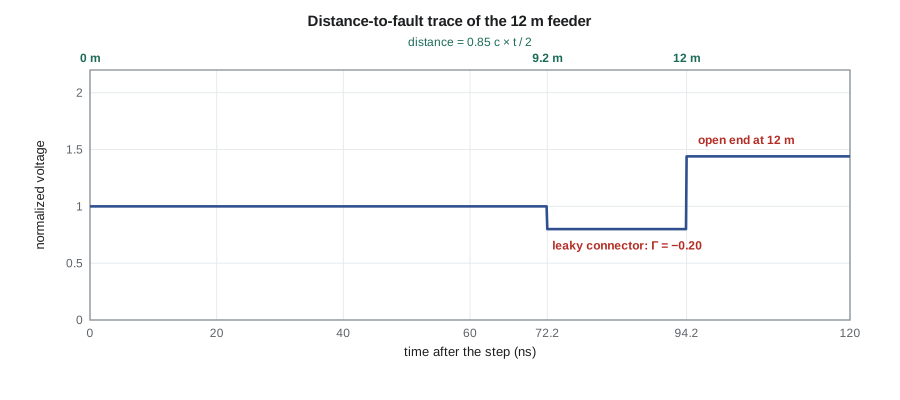
A time-domain reflectometer, or TDR, launches a fast step or pulse into a cable and records the voltage at its input. Each discontinuity along the cable sends back a reflection whose sign and size reveal what it is and whose delay reveals where it is, distance being half the delay times the propagation velocity. A short circuit gives a step down to zero, an open circuit a step up, a crushed section of cable with lower impedance a dip, a series resistance or corroded connector a rise, a shunt leakage from water a dip. Many modern network analyzers and cable and antenna analyzers compute the same information from a frequency sweep, a mode often called distance-to-fault.
Worked problem
Finding the leaky connector
A year after installation, one cabinet's link margin has fallen by about 3 dB. A technician connects a cable and antenna analyzer in distance-to-fault mode to the feeder at the radio end. The trace shows a reflection of −0.20 at 72.2 ns and a larger reflection at 94.2 ns. The cable's velocity factor is 0.85. Where are the faults, and what are they?
Show solution
- \[v = 0.85 \times 2.998\times10^8 = 2.548\times10^8\ \text{m/s}\]
- \[d_1 = \frac{v\,t_1}{2} = \frac{2.548\times10^8 \times 72.2\times10^{-9}}{2} = 9.20\ \text{m}\]
- \[d_2 = \frac{2.548\times10^8 \times 94.2\times10^{-9}}{2} = 12.0\ \text{m}\]
- A shunt leakage of 100 Ω across a 50 Ω line gives Γ = (33.3 − 50)/(33.3 + 50) = −0.20, matching the first reflection.
Answer: A fault at 9.2 m that looks like a shunt leak, the size expected from water in a connector, and the antenna at 12.0 m (disconnected for the test, so it shows as an open). Leo's installation records place an in-line connector where the cable passes through the mast-arm clamp, 9.2 m from the cabinet. The fix is to replace and weatherproof that connector, and the field-installation instructions gain a line about self-amalgamating tape over every outdoor connector.
Loss and the ABCD matrix
On a lossy line, Γ shrinks by e^{−2αℓ} as well as rotating, so the point on the Smith chart spirals inward toward the centre as you move toward the generator, the graphical form of lesson 9's warning that loss hides a bad load. For chains of line sections and lumped elements, the ABCD or transmission matrix of each part multiplies to give the whole. For a line section it is [cosh γℓ, Z₀ sinh γℓ; sinh γℓ/Z₀, cosh γℓ], the same matrix lesson 8 used for a slab of material, because a plane wave crossing a layer and a voltage wave on a line obey the same equations. Circuit simulators that handle transmission lines use exactly this matrix, and you can use it to analyse the feeder, a jumper, a lightning arrester and the matching network as a single chain.
Common mistakes
MistakeExpecting the VSWR to change along a lossless line.
Instead|Γ| is constant; only its phase rotates, and the impedance moves round a constant-VSWR circle.
MistakeMatching at the radio end of a long feeder.
InsteadThe impedance there depends on the exact electrical length and frequency; match at the load.
MistakeConverting TDR delay to distance with the free-space speed.
InsteadUse the cable's velocity factor and divide the round-trip time by two.
MistakeAssuming a quarter-wave transformer matches any load.
InsteadIt matches a real load; move a complex load to a real-impedance point first or use a stub or L-network.
Summary and key terms
- Z_in = Z₀(Z_L + jZ₀ tan βℓ)/(Z₀ + jZ_L tan βℓ); Γ rotates by −2βℓ along a lossless line.
- Shorted and open stubs act as reactances; a quarter wave inverts impedance and a half wave repeats it.
- The Smith chart maps normalized impedance onto the Γ plane; moving along a line is a rotation about the centre.
- Quarter-wave transformers, single stubs and L-networks match a load to Z₀; bandwidth narrows as the impedance ratio grows.
- Step responses bounce between mismatched ends; matching either end stops the bouncing.
- TDR and distance-to-fault locate discontinuities from the sign, size and delay of their reflections.
- Input impedance
- The impedance seen looking into a line toward its load.
- Stub
- A short- or open-circuited section of line used as a reactance.
- Quarter-wave transformer
- A λ/4 section of impedance √(Z₀R_L) that matches R_L to Z₀.
- Smith chart
- A chart of the reflection-coefficient plane overlaid with normalized impedance coordinates.
- Constant-VSWR circle
- The circle about the Smith chart centre on which a load moves along a lossless line.
- Bounce diagram
- A distance–time diagram of reflections on a line after a step.
- Time-domain reflectometry
- Locating discontinuities on a line from the reflections of a fast step or pulse.
- ABCD matrix
- A two-port matrix relating input voltage and current to output voltage and current.
Practice problems
Work each problem on paper first, then reveal the answer to check.
Find Z_in of a 50 Ω line λ/4 long terminated in 25 Ω.
Show answer
100 Ω.
What length of short-circuited 50 Ω line gives +j50 Ω?
Show answer
tan βℓ = 1, ℓ = λ/8.
Design a quarter-wave transformer to match a 12.5 Ω load to 50 Ω.
Show answer
Z_T = 25 Ω, λ/4 long.
A load has Γ = 0.3∠60°. What is Γ λ/8 toward the generator?
Show answer
0.3∠−30°.
A TDR on cable with velocity factor 0.66 shows a short at 151 ns. Where is it?
Show answer
0.66 × 3 × 10⁸ × 151 × 10⁻⁹ / 2 = 15.0 m.
A 5 V step from a 50 Ω source enters a 50 Ω line ending in an open circuit. What is the final voltage, and how many reflections occur?
Show answer
2.5 V launched, doubling to 5 V at the open; the matched source absorbs the return, so one reflection.
Lesson quiz · 5 questions
Score 60% or more to complete this lesson.
Create a free account to save your progress, take quizzes and earn a certificate.