
ELE-280 · Lesson 6 of 12 · 25 min
Oscilloscopes I: triggering, timebase and probes
A multimeter gives one number. An oscilloscope shows how a voltage changes with time, and that picture reveals things no meter can: the shape of a ripple waveform, the ringing on a logic edge, the delay between a button press and a response, a glitch that happens once in a thousand cycles. Almost every modern bench scope is a digital storage oscilloscope, which samples the input with a fast analog-to-digital converter, stores the samples in memory and draws them on a screen. This lesson covers the controls you use every time: vertical scale and coupling, the timebase, triggering, the automatic measurements and the passive probe, including the compensation step that many people skip.
Amara asks Leo to look at three signals on the controller board: the 24 V rail's ripple, the 5 V logic clock driving the shift registers that select the signal heads, and the output of the push-button debouncer when the button is pressed. Each one needs a different setup, and each one teaches a control.
The display and the vertical controls
The screen is a grid, usually ten divisions across and eight divisions high. The vertical scale, in volts per division, sets how many volts each division represents, and the position control moves the trace up or down. The input coupling selects what reaches the converter: DC coupling passes the whole signal, including its DC level; AC coupling inserts a series capacitor that blocks DC and passes only the changing part, with a low-frequency corner of a few hertz; and ground disconnects the input to show where zero is. To see 200 mV of ripple riding on a 24 V rail, DC coupling at 50 mV per division would put the trace far off the screen. AC coupling removes the 24 V and lets you expand the ripple to fill the screen.
Because the converter has a fixed number of bits, usually 8 on a general-purpose scope and 10 to 12 on high-resolution ones, the vertical scale sets the resolution too. An 8-bit converter spread over eight divisions has 256 levels, so at 1 V per division each level is about 31 mV. Small details on a large signal disappear into the quantization. Adjust the vertical scale so the signal fills most of the screen; this uses the converter's full range and gives the most precise measurements.
The timebase and acquisition memory
The horizontal scale, in seconds per division, sets the time window: at 1 ms per division, ten divisions show 10 ms. The horizontal position control moves the window relative to the trigger point. Behind the scenes, the scope has a maximum sample rate, for example 1 GSa/s, and a memory depth, the number of samples it can store per acquisition, for example 10 Mpoints. The sample rate actually used is the memory depth divided by the time window, up to the maximum. Over a long window, a scope with shallow memory has to reduce its sample rate, and fast details can be lost or aliased, a problem lesson 7 returns to. Deep memory lets you capture a long window and still zoom in on fast events.
Triggering: making the picture stand still
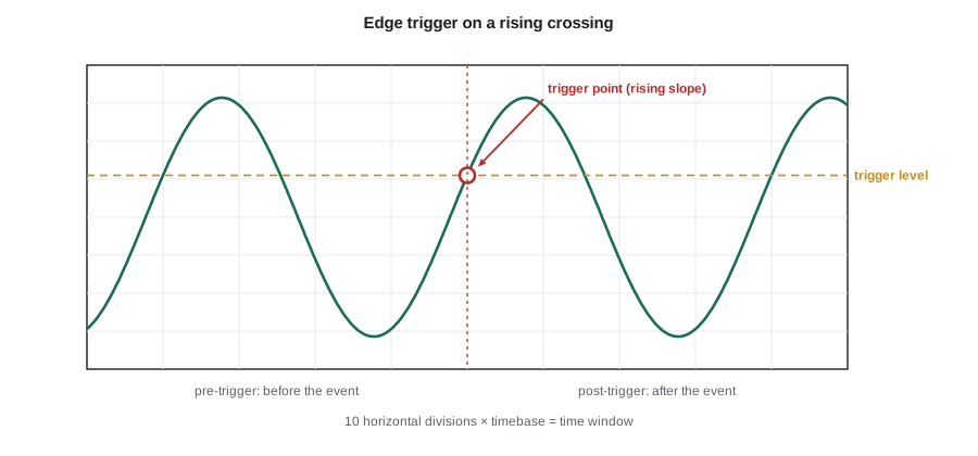
A repeating waveform only looks stable on screen if every sweep starts at the same point in its cycle. The trigger decides that point. The simplest and most used is the edge trigger: start the sweep when the signal crosses a set level in a set direction, rising or falling. Set the level in the middle of the waveform, choose the slope, and a repeating signal locks in place. If the level is above the waveform's peak or below its trough, no trigger occurs, and the scope either waits forever or free-runs and shows a smeared mess, depending on the trigger mode.
| Trigger mode | Behaviour | Use |
|---|---|---|
| Auto | Triggers on the set condition, but sweeps anyway if no trigger occurs for a short time | Finding a signal, seeing DC levels |
| Normal | Sweeps only when the trigger condition occurs; otherwise holds the last trace | Stable display of occasional or low-rate signals |
| Single | Captures one triggered acquisition and stops | One-time events: a power-up, a button press, a fault |
Single mode is the one beginners forget, and it is the one that captures the most informative events. A button press, a power-up surge, a fault that happens once a minute: none of them repeat in a way that auto or normal mode can hold. Set the trigger level and slope where the event should cross, press Single, then cause the event. The scope captures it, stops, and keeps it on screen for measurement. Because the trigger point is in the middle of the record by default, you also see what led up to it. Beyond edge triggers, modern scopes offer pulse-width triggers, which fire on a pulse shorter or longer than a set time and catch glitches; runt triggers, which fire on a pulse that crosses one level but not another; and serial-bus triggers that decode protocols such as I²C, SPI and UART and trigger on a particular message.
Worked problem
Catching a switch bounce
The push-button input should go from 5 V to 0 V when pressed. Leo wants to see whether the contacts bounce and how long the debounce circuit takes to settle. How should he set up the scope?
Show solution
- Connect the probe to the switch side of the debouncer, before the RC filter, so that bounces are visible.
- Set the vertical scale to 1 V per division with DC coupling and position zero near the bottom of the screen, so 0 to 5 V fills five divisions.
- Contact bounce typically lasts from a few hundred microseconds to a few milliseconds, so set the timebase to 1 ms per division for a 10 ms window.
- Choose an edge trigger, falling slope, level 2.5 V, and Single mode. Press the button.
Answer: The capture shows the falling edge at the centre of the screen, followed by several bounces back toward 5 V over about 1.5 ms before the line stays low. A second channel on the debouncer output shows a smooth exponential fall with no bounces, which crosses the logic threshold once. The measurement tells Amara the RC time constant is long enough.
Automatic measurements and cursors
Digital scopes measure waveforms automatically: frequency, period, peak-to-peak and RMS amplitude, mean, rise and fall time, pulse width, duty cycle, overshoot and the delay between channels. These are quick and usually more precise than reading the grid by eye, but they compute what they are told on whatever is on screen. A frequency measurement on a noisy signal with only part of a cycle on screen will be wrong; an RMS measurement over a window that does not contain a whole number of cycles will be slightly off. Rise time is conventionally measured between the 10 % and 90 % points of the transition, so the scope needs a clean top and bottom level to find them. Cursors, adjustable lines you place on the screen, let you measure any two points by hand and are useful when the automatic measurement is confused.
The passive probe
The standard probe supplied with a scope is a 10:1 (10X) passive probe. The scope input is about 1 MΩ in parallel with 10 to 20 pF, and the probe puts a 9 MΩ resistor in its tip so that, together with the scope's 1 MΩ, the signal is divided by ten and the circuit sees 10 MΩ instead of 1 MΩ. The cable and scope input add capacitance, which would turn that 9 MΩ into a low-pass filter. The probe therefore includes an adjustable compensation capacitor that makes the divider's time constants equal at the tip and at the scope end, so the division ratio is ten at every frequency. Seen from the circuit, a 10X probe looks like 10 MΩ in parallel with roughly 10 to 15 pF.
A 1X probe, or a probe switched to 1X, connects the circuit straight to the scope input through the cable. It gives full sensitivity, which helps with millivolt signals, but presents about 1 MΩ and the full cable and input capacitance, often 50 pF or more, and its bandwidth is typically only a few megahertz. For almost all general work, use 10X, and check that the scope's channel setting matches the probe so the displayed volts are right. Many probes identify themselves to the scope automatically; others need the attenuation set in the channel menu.
Compensating the probe
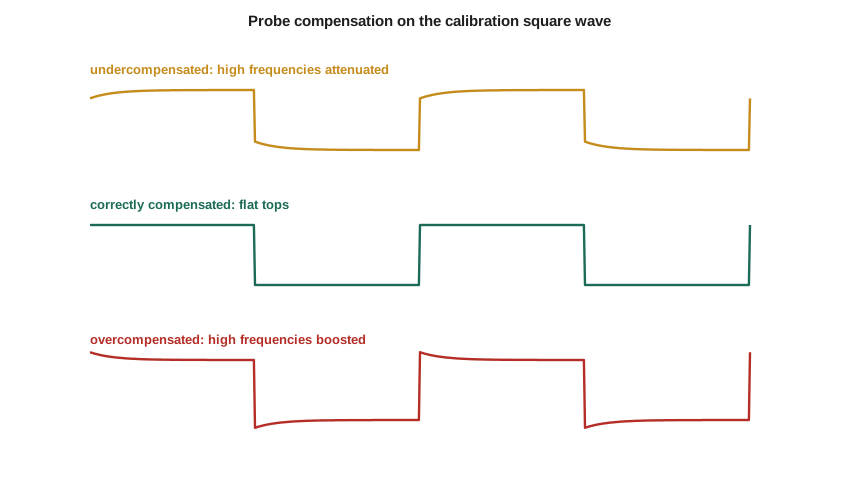
Every time a probe is connected to a different scope input, its compensation should be checked. Each scope has a calibration output on the front panel, a square wave of about 1 kHz and a few volts. Connect the probe to it, display a few cycles, and adjust the small screw on the probe until the square wave has flat tops. An undercompensated probe rounds the corners, attenuating high frequencies; an overcompensated probe shows peaks on the leading edges, boosting them. Either error changes rise-time measurements and the apparent amplitude of fast signals by many percent.
# Probe compensation: response of a 10X divider with mismatched capacitors to a step
import math
Rtip, Rin = 9e6, 1e6
Cin = 20e-12 + 80e-12          # scope input plus cable
Cc_correct = Rin * Cin / Rtip   # tip capacitor that balances the divider
print(f"Correct tip capacitance: {Cc_correct*1e12:.2f} pF")

def step_response(Ctip, t):
    # Divider of two RC sections: initial value set by capacitors, final by resistors
    v0 = Ctip / (Ctip + Cin)            # high-frequency ratio (capacitive divider)
    vinf = Rin / (Rin + Rtip)           # low-frequency ratio (resistive divider)
    tau = (Rtip * Rin / (Rtip + Rin)) * (Ctip + Cin)
    return vinf + (v0 - vinf) * math.exp(-t / tau), tau

for label, c in (("under", 0.7 * Cc_correct), ("correct", Cc_correct), ("over", 1.3 * Cc_correct)):
    v0, tau = step_response(c, 0.0)
    v_late, _ = step_response(c, 5 * tau)
    print(f"{label:8s} Ctip = {c*1e12:5.2f} pF: edge starts at {10*v0:.3f}, settles to {10*v_late:.3f} "
f"(tau = {tau*1e6:.1f} us)")Correct tip capacitance: 11.11 pF under Ctip = 7.78 pF: edge starts at 0.722, settles to 0.998 (tau = 97.0 us) correct Ctip = 11.11 pF: edge starts at 1.000, settles to 1.000 (tau = 100.0 us) over Ctip = 14.44 pF: edge starts at 1.262, settles to 1.002 (tau = 103.0 us)
The program shows the physics behind the three pictures. At the instant of a step, the divider ratio is set by the capacitors; long after, by the resistors. When the capacitive ratio is too small, the edge starts low and creeps up; when it is too large, the edge starts high and decays. Only when R_tip·C_tip equals R_in·C_in do the two ratios match, and the edge is a clean step. The settling time constant, around a hundred microseconds, is why the error is easy to see on a 1 kHz calibration square wave.
The ground lead
The probe's ground lead, the short wire with an alligator clip, connects the probe's shield to the circuit's ground. It is part of the measurement loop, and its inductance, roughly 1 nH per millimetre, forms a resonant circuit with the probe's input capacitance. On slow signals that does not matter. On fast edges, a 15 cm ground lead can add ringing at a few hundred megahertz that is not in the circuit at all. For fast signals, replace the long lead with the short spring ground tip that comes with the probe, and touch it to a ground pad right beside the signal point. Never clip the ground lead to anything that is not at ground potential; lesson 7 explains why on a mains-powered scope.
Worked problem
Choosing settings for the ripple
Leo wants to measure the 24 V rail's ripple, about 0.6 V peak-to-peak at 120 Hz from the full-wave rectifier, on a scope with an 8-bit converter. Compare DC coupling at 5 V per division with AC coupling at 200 mV per division.
Show solution
- At 5 V per division over eight divisions, each converter level is 40 V / 256 ≈ 156 mV, so the 0.6 V ripple spans only about four levels and looks like a staircase.
- With AC coupling, the DC is removed. At 200 mV per division, the ripple fills three divisions and each level is 1.6 V / 256 ≈ 6.3 mV.
- A timebase of 2 ms per division shows 20 ms, about two and a half ripple cycles. Trigger on the rising edge of the ripple at its midpoint.
Answer: AC coupling at 200 mV per division resolves the ripple about 25 times more finely and shows its sawtooth shape: a steep rise while the rectifier charges the capacitor and a slow linear fall as the load discharges it. The AC coupling's low-frequency corner, a few hertz, is far below 120 Hz, so it does not distort the ripple.
Common mistakes
MistakeLeaving the trigger level outside the waveform.
InsteadSet the level between the signal's minimum and maximum; use Auto mode to find the signal first.
MistakeTrying to see a one-time event in Auto mode.
InsteadUse Single mode with an edge or pulse trigger set where the event will cross.
MistakeSkipping probe compensation.
InsteadCheck the probe on the calibration output whenever it is moved to a different scope or channel.
MistakeUsing a 1X probe for fast or high-impedance signals.
InsteadUse 10X for general work; 1X has low bandwidth and loads the circuit heavily.
MistakeUsing the long ground lead on fast edges.
InsteadUse the spring ground tip and a nearby ground point; long leads add ringing that is not in the circuit.
Summary and key terms
- A digital scope samples the input with an ADC, stores it in memory and draws it on a grid of divisions.
- Vertical scale, position and coupling set what you see; fill the screen to use the converter's full resolution.
- Timebase and memory depth set the window and the sample rate actually used.
- The trigger fixes each sweep to the same point; edge triggers suit repeating signals and Single mode captures one-time events.
- Automatic measurements are convenient but compute only what is on screen; cursors give manual control.
- A 10X passive probe presents about 10 MΩ and 10 to 15 pF and must be compensated on the calibration output; short grounds matter on fast edges.
- Timebase
- The horizontal scale of an oscilloscope, in seconds per division.
- Trigger
- The condition that starts an oscilloscope acquisition, so repeated sweeps line up.
- Edge trigger
- A trigger that fires when the signal crosses a set level in a set direction.
- Memory depth
- The number of samples an oscilloscope stores per acquisition.
- AC coupling
- An input setting that blocks the DC component with a series capacitor.
- Probe compensation
- Adjustment of a passive probe's capacitor so its division ratio is the same at all frequencies.
- Rise time
- The time a signal takes to go from 10 % to 90 % of its transition.
Practice problems
Work each problem on paper first, then reveal the answer to check.
At 500 µs per division, how long is the full screen window?
Show answer
5 ms.
A scope with 1 Mpoint of memory shows a 100 ms window. What sample rate does it use if its maximum is 1 GSa/s?
Show answer
10 MSa/s.
An 8-bit scope is set to 0.5 V per division. What is the size of one converter level?
Show answer
4 V / 256 ≈ 15.6 mV.
A square wave on the calibration output shows spikes on its leading edges. What is wrong?
Show answer
The probe is overcompensated; turn the adjustment the other way.
Which trigger mode would you use to capture the 24 V rail at power-up?
Show answer
Single, with a rising edge trigger at about half the final voltage.
What does a 10X probe look like to the circuit?
Show answer
About 10 MΩ in parallel with roughly 10 to 15 pF.
Lesson quiz · 5 questions
Score 60% or more to complete this lesson.
Create a free account to save your progress, take quizzes and earn a certificate.