
ELE-280 · Lesson 3 of 12 · 23 min
Uncertainty and error analysis
Lesson 2 showed that every reading comes with a range of doubt. This lesson makes that doubt quantitative. Uncertainty analysis answers two questions that come up in every lab: how well do I know this measured value, and how well do I know a result calculated from several measured values? The method used here follows the international Guide to the Expression of Uncertainty in Measurement, usually called the GUM, which is the basis of calibration certificates and of uncertainty statements in standards and test reports in Canada, the United States and most other countries. You do not need its full machinery for a teaching lab, but its core ideas fit on a page and they are used everywhere.
Amara gives Leo a concrete job. The pedestrian controller drives each LED signal head through a 2.2 Ω current-sense resistor, and the firmware estimates the LED current from the voltage across it. Leo must measure that voltage repeatedly, compute the current and the power dissipated in the resistor, and state both with uncertainties so that Amara can decide whether the resistor's 0.5 W rating leaves enough margin.
Error and uncertainty
The error of a measurement is the difference between the measured value and the true value. We never know it exactly, because we never know the true value exactly; if we did, we would not need to measure. Uncertainty is our quantitative estimate of how large the error could reasonably be. A result written as 0.418 ± 0.004 V says that the true value very probably lies within that interval, and the statement should also say how probable. The GUM expresses each source of uncertainty as a standard uncertainty, written u, which has the meaning of a standard deviation. Standard uncertainties from different sources are then combined, and the result is multiplied by a coverage factor to give an interval with a stated level of confidence.
Type A: uncertainty from repeated readings
A Type A evaluation uses statistics on repeated measurements. Take n independent readings x₁ to xₙ. Their mean is the best estimate of the value, and their experimental standard deviation s describes the scatter of individual readings. The uncertainty of the mean is smaller than the scatter of single readings, because averaging reduces random error: it is the standard deviation of the mean, s/√n.
The divisor n − 1 rather than n in s corrects for the fact that the deviations are measured from the sample mean rather than the unknown true mean. For small n, the estimate s is itself uncertain, which is why a mean of only three readings deserves a larger coverage factor than a mean of fifty. With ten or more readings the difference is modest, and teaching labs usually ignore it, but it is worth knowing that a standard deviation from three readings can easily be off by a factor of two.
Type B: uncertainty from other information
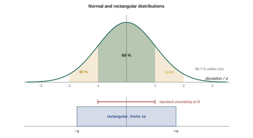
A Type B evaluation uses everything except repeated readings: the instrument specification, a calibration certificate, a resistor tolerance, the resolution of the display, or experience. The trick is to turn each of those into a standard uncertainty. When a specification gives limits ±a and nothing else is known about where in that range the error lies, the GUM treats every value in the range as equally likely, a rectangular distribution, whose standard deviation is a/√3. A meter specified to ±0.017 V therefore contributes about 0.0098 V of standard uncertainty. A calibration certificate that reports an expanded uncertainty U with coverage factor k = 2 contributes U/2. The display's resolution, one count of width δ, is a rectangle of half-width δ/2, contributing δ/(2√3), which is usually negligible when the accuracy specification already covers it.
Combining uncertainties
When independent sources each contribute a standard uncertainty to the same quantity, they combine in quadrature, as the square root of the sum of the squares. Adding them directly would assume that every source is at its worst limit in the same direction at once, which is unlikely for independent errors. The root-sum-square, or RSS, gives the combined standard uncertainty u_c.
Finally, the expanded uncertainty U = k·u_c gives an interval x̄ ± U. With k = 2 and a roughly normal result, the interval has a coverage probability of about 95 %, and that is the usual choice on calibration certificates and in reports. Always state k. A reader cannot interpret ±0.004 V without knowing whether it is one standard uncertainty, a 95 % interval or a worst-case limit.
Worked problem
Uncertainty of the sense-resistor voltage
Leo takes ten readings of the voltage across the 2.2 Ω resistor with the LED on: 0.4184, 0.4179, 0.4188, 0.4181, 0.4186, 0.4183, 0.4177, 0.4185, 0.4182 and 0.4180 V. The meter's specification on its 6 V range is ±(0.05 % + 5 counts) with one count = 0.1 mV. Find the mean, the Type A and Type B standard uncertainties, the combined standard uncertainty and the expanded uncertainty with k = 2.
Show solution
- The mean is x̄ = 0.41825 V and the experimental standard deviation of the ten readings is s ≈ 0.000337 V.
- \[u_A = \frac{s}{\sqrt{n}} = \frac{0.000337}{\sqrt{10}} \approx 0.000107\ \text{V}\]
- The specification limit is a = 0.0005 × 0.41825 + 5 × 0.0001 = 0.000209 + 0.0005 = 0.000709 V. Treating it as rectangular:
- \[u_B = \frac{a}{\sqrt{3}} = \frac{0.000709}{1.732} \approx 0.000409\ \text{V}\]
- \[u_c = \sqrt{0.000107^2 + 0.000409^2} \approx 0.000423\ \text{V}, \qquad U = 2u_c \approx 0.00085\ \text{V}\]
Answer: V = 0.4183 ± 0.0008 V (k = 2). The meter's specification dominates; taking a hundred readings instead of ten would barely change the result, because averaging cannot reduce the Type B term.
Propagating uncertainty through a calculation
Most lab results are calculated from several measurements: a current from a voltage and a resistance, a power from a current and a voltage, a time constant from a resistance and a capacitance. If y = f(x₁, x₂, …) and the inputs are independent, each input's standard uncertainty contributes to y in proportion to how sensitive y is to that input, which is the partial derivative ∂f/∂xᵢ, called the sensitivity coefficient. The contributions then combine in quadrature.
Two shortcuts cover most lab calculations. For sums and differences, y = x₁ ± x₂, the absolute uncertainties combine in quadrature. For products, quotients and powers, y = c·x₁ᵃ·x₂ᵇ, the relative uncertainties combine in quadrature, each multiplied by its exponent: (u_y/y)² = (a·u₁/x₁)² + (b·u₂/x₂)². A quantity that appears squared therefore contributes twice its relative uncertainty, which is why the power P = V²/R is more sensitive to the voltage than to the resistance.
| Relationship | Combined standard uncertainty |
|---|---|
| y = x₁ + x₂ or x₁ − x₂ | u_y = √(u₁² + u₂²) |
| y = c·x (c exact) | u_y = |c|·u_x |
| y = x₁·x₂ or x₁/x₂ | u_y/|y| = √((u₁/x₁)² + (u₂/x₂)²) |
| y = xⁿ | u_y/|y| = |n|·u_x/|x| |
| y = ln x | u_y = u_x/|x| |
One warning: the quadrature rule assumes the inputs are independent. If two readings are taken with the same meter on the same range, their calibration errors are correlated, and some of the error cancels in a ratio or adds in a sum. A classic example is measuring the gain of an amplifier as the ratio of two voltages read on the same meter and range: the meter's gain error divides out, and the uncertainty of the ratio is much smaller than the quadrature sum of the two readings would suggest. The GUM handles this with covariance terms. For lab work, it is enough to notice when correlation is likely and to say which way it pushes the result.
# Type A + Type B uncertainty for the sense-resistor voltage, then propagation to I and P
import math, statistics as st
v = [0.4184, 0.4179, 0.4188, 0.4181, 0.4186, 0.4183, 0.4177, 0.4185, 0.4182, 0.4180]
n = len(v); vbar = st.mean(v); s = st.stdev(v)
uA = s / math.sqrt(n)
a = 0.0005 * vbar + 5 * 0.0001          # meter spec limit on the 6 V range
uB = a / math.sqrt(3)
uV = math.hypot(uA, uB)
print(f"V = {vbar:.5f} V, s = {s*1e3:.3f} mV, uA = {uA*1e3:.3f} mV, uB = {uB*1e3:.3f} mV, uc = {uV*1e3:.3f} mV")

R = 2.2; uR = 0.01 * R / math.sqrt(3)   # 1 % tolerance resistor, rectangular
I = vbar / R
uI = I * math.hypot(uV / vbar, uR / R)
P = vbar**2 / R
uP = P * math.hypot(2 * uV / vbar, uR / R)
print(f"I = {I*1e3:.2f} mA +/- {2*uI*1e3:.2f} mA (k=2)")
print(f"P = {P*1e3:.2f} mW +/- {2*uP*1e3:.2f} mW (k=2); rating 500 mW, margin x{0.5/P:.1f}")

# Monte Carlo check of the propagation for P
import random
random.seed(1)
samples = []
for _ in range(100000):
    vv = random.gauss(vbar, uV)
    rr = R * (1 + random.uniform(-0.01, 0.01))
    samples.append(vv * vv / rr)
print(f"Monte Carlo: P mean {st.mean(samples)*1e3:.2f} mW, std {st.stdev(samples)*1e3:.3f} mW "
f"vs propagated {uP*1e3:.3f} mW")V = 0.41825 V, s = 0.337 mV, uA = 0.107 mV, uB = 0.409 mV, uc = 0.423 mV I = 190.11 mA +/- 2.23 mA (k=2) P = 79.52 mW +/- 0.97 mW (k=2); rating 500 mW, margin x6.3 Monte Carlo: P mean 79.52 mW, std 0.486 mW vs propagated 0.486 mW
The program confirms the hand result and adds the current and power. The 1 % resistor tolerance is now the largest single contributor to the current's uncertainty, ahead of the meter. The power is about 80 mW, so the 0.5 W resistor runs at about a sixth of its rating; Amara is satisfied. The Monte Carlo section draws a hundred thousand random combinations of voltage and resistance, computes the power for each, and finds the same spread as the formula. Monte Carlo simulation is the GUM's recommended method when the formula is non-linear or the inputs are far from normal, and with a few lines of code it is often easier than taking derivatives.
Uncertainty budgets
An uncertainty budget is a table that lists each source, its type, its standard uncertainty, its sensitivity coefficient and its contribution to the result. It shows at a glance which source dominates, and therefore where effort will pay. If the budget shows that the resistor tolerance dominates, buying a better meter is wasted money; measuring the resistor itself with a four-wire ohmmeter, as lesson 8 describes, would help far more.
| Source | Type | Standard uncertainty | Contribution to I |
|---|---|---|---|
| Voltage scatter (10 readings) | A | 0.11 mV | 0.05 mA |
| Meter specification | B (rectangular) | 0.41 mV | 0.19 mA |
| Resistor tolerance, 1 % | B (rectangular) | 0.0127 Ω | 1.10 mA |
| Combined | 1.12 mA | ||
| Expanded, k = 2 | 2.2 mA |
Worked problem
Is the difference significant?
The firmware reports an LED current of 186 mA, while Leo's measurement gives 190.1 ± 2.2 mA (k = 2). Is the firmware's value inconsistent with the measurement?
Show solution
- The difference is 190.1 − 186 = 4.1 mA.
- The firmware value has its own uncertainty, which Leo does not know yet. Against the measurement alone, the difference is about 4.1 / 1.12 ≈ 3.7 standard uncertainties.
- A difference of more than about two combined standard uncertainties is usually treated as significant.
Answer: The difference is likely real, not measurement noise. Leo should look for a systematic cause, such as the firmware using the nominal 2.2 Ω value while the actual resistor is 1 % high, or an offset in the microcontroller's analog-to-digital converter.
Common mistakes
MistakeAdding all uncertainty contributions directly.
InsteadCombine independent standard uncertainties in quadrature; direct addition gives a worst case, which should be labelled as such.
MistakeUsing the spread of readings as the only uncertainty.
InsteadInclude Type B sources such as the instrument specification and component tolerances; they often dominate.
MistakeDividing the standard deviation by √n and calling that the uncertainty of a single reading.
Insteads/√n is the uncertainty of the mean; a single reading has uncertainty s.
MistakeForgetting the exponent when propagating a squared quantity.
InsteadFor y = x², the relative uncertainty doubles.
MistakeStating ± without saying what it means.
InsteadGive the coverage factor, for example k = 2 for about 95 %, or say that it is a worst-case limit.
Summary and key terms
- Uncertainty is a quantitative estimate of the possible error; the GUM expresses each source as a standard uncertainty with the meaning of a standard deviation.
- Type A uncertainty comes from statistics of repeated readings; the uncertainty of a mean is s/√n.
- Type B uncertainty comes from specifications, certificates and tolerances; limits ±a with no other information give u = a/√3.
- Independent standard uncertainties combine as the root-sum-square, and the expanded uncertainty is U = k·u_c, usually with k = 2.
- Propagation uses sensitivity coefficients; relative uncertainties combine for products and quotients, scaled by exponents.
- An uncertainty budget shows which source dominates, and Monte Carlo simulation checks non-linear propagation.
- Standard uncertainty
- An uncertainty expressed as a standard deviation.
- Type A evaluation
- Evaluation of uncertainty by statistical analysis of repeated observations.
- Type B evaluation
- Evaluation of uncertainty by other means, such as specifications, certificates or tolerances.
- Combined standard uncertainty
- The root-sum-square of the contributions of all uncertainty sources to a result.
- Expanded uncertainty
- The combined standard uncertainty multiplied by a coverage factor k to give an interval with a stated coverage probability.
- Sensitivity coefficient
- The partial derivative of a result with respect to an input, describing how strongly that input affects the result.
- Uncertainty budget
- A table listing each uncertainty source and its contribution to the combined uncertainty.
- GUM
- The Guide to the Expression of Uncertainty in Measurement, the international reference for uncertainty analysis.
Practice problems
Work each problem on paper first, then reveal the answer to check.
Five readings have s = 0.40 mV. What is the standard uncertainty of their mean?
Show answer
0.40/√5 ≈ 0.18 mV.
A resistor is marked 1 kΩ ± 5 %. What standard uncertainty does that tolerance give, assuming a rectangular distribution?
Show answer
50 Ω/√3 ≈ 29 Ω.
Two independent contributions are 3 mV and 4 mV. Find the combined standard uncertainty.
Show answer
5 mV.
P = V²/R, with V known to 0.3 % and R to 0.5 % (both standard uncertainties). Find the relative uncertainty of P.
Show answer
√(0.6² + 0.5²) ≈ 0.78 %.
A calibration certificate gives U = 0.02 Ω with k = 2. What standard uncertainty should you use?
Show answer
0.01 Ω.
Why can measuring an amplifier's gain with the same meter on the same range give a smaller uncertainty than the quadrature rule predicts?
Show answer
The meter's gain error affects both readings in the same way and divides out of the ratio; the errors are correlated.
Lesson quiz · 5 questions
Score 60% or more to complete this lesson.
Create a free account to save your progress, take quizzes and earn a certificate.