Probabilistic classifiers: naive Bayes and discriminant analysis

There are two ways to build a probabilistic classifier. A discriminative model, such as logistic regression, models \(P(y \mid \mathbf{x})\) directly: it learns a boundary between classes and never asks how the inputs themselves are distributed. A generative model learns how each class produces its inputs, a class-conditional density \(p(\mathbf{x} \mid y)\), together with the class prior \(P(y)\), and then classifies with Bayes' rule:

The denominator is the same for every class, so the predicted class is \(\arg\max_k p(\mathbf{x} \mid y = k) P(y = k)\). Generative classifiers can do things discriminative ones cannot: generate synthetic examples, detect inputs unlike anything seen in training (low \(p(\mathbf{x})\)), handle missing features by marginalizing them out, and incorporate prior knowledge about how data are produced. They also tend to learn from fewer examples. Their weakness is that modelling the whole input distribution is harder than modelling a boundary, and errors in that model become errors in classification.

This lesson develops the two most important generative classifiers: naive Bayes, which assumes features are conditionally independent given the class, and Gaussian discriminant analysis, which assumes each class is a multivariate Gaussian. CMPUT-366's lesson on Bayesian networks provides the probabilistic background: naive Bayes is the simplest Bayesian network, a class node with an arrow to every feature. AI-320 develops richer generative models.

The naive Bayes assumption

With d binary features, the class-conditional distribution \(p(\mathbf{x} \mid y)\) has \(2^d - 1\) free parameters per class, far too many to estimate from data. Naive Bayes makes a drastic simplifying assumption: given the class, the features are independent, so

and the parameters number only d per class. The assumption is almost always false. In a spam filter, the words free and prize are not independent given that a message is spam. Yet naive Bayes often classifies well, for a reason Pedro Domingos and Michael Pazzani analysed in 1997: classification needs only the correct ordering of the class posteriors, not accurate values, and the errors introduced by the independence assumption often push all classes in similar directions. Its probability estimates, however, are typically far too extreme, because correlated features are counted as independent pieces of evidence; if they matter, they must be recalibrated (lesson 9).

Naive Bayes for text

Naive Bayes has a long history in text classification, from Maron's 1961 work on automatic indexing to the spam filters popularized by Paul Graham's 2002 essay A Plan for Spam. The multinomial model treats a document as a bag of words: it ignores word order and models the word counts. The probability of word w in class k is estimated as its share of all words in class k's training documents. A word that never appears in a class's training documents would get probability zero and veto that class for any document containing it, however strong the other evidence. Laplace (add-one) smoothing prevents this by adding a pseudo-count \(\alpha\) to every word:

where \(\lvert V \rvert\) is the vocabulary size. Smoothing is the maximum a posteriori estimate under a Dirichlet prior, and \(\alpha\) is a regularization hyperparameter like the \(\lambda\) of ridge regression. Multiplying hundreds of small probabilities underflows floating-point arithmetic, so implementations add log probabilities instead, and convert back with the log-sum-exp trick only when a probability is needed.

# Multinomial naive Bayes from scratch on a tiny invented set of messages.
import math
from collections import Counter
train = [("win a free prize now", "spam"), ("free money claim your prize", "spam"),
         ("limited offer win cash now", "spam"), ("claim free cash offer", "spam"),
         ("meeting moved to tuesday", "ham"), ("can you send the lab report", "ham"),
         ("lunch on tuesday with the team", "ham"), ("report due friday please review", "ham"),
         ("free pizza at the team meeting", "ham")]
classes = ["spam", "ham"]
vocab = sorted({w for text, _ in train for w in text.split()})
counts = {c: Counter() for c in classes}; docs = Counter()
for text, c in train:
    counts[c].update(text.split()); docs[c] += 1

def log_posterior(text, alpha=1.0):
    scores = {}
    for c in classes:
        total = sum(counts[c].values())
        s = math.log(docs[c] / len(train))                   # log prior
        for w in text.split():
            if w in vocab:                                   # ignore words never seen in training
                s += math.log((counts[c][w] + alpha) / (total + alpha * len(vocab)))
        scores[c] = s
    return scores

for msg in ["claim your free prize", "team meeting on friday", "free lunch with the team"]:
    s = log_posterior(msg)
    z = max(s.values()); p_spam = math.exp(s["spam"] - z) / sum(math.exp(v - z) for v in s.values())
    print(f"{msg!r:28} -> {max(s, key=s.get):4}  P(spam) = {p_spam:.3f}")
print(f"vocabulary size {len(vocab)}; P(word='free' | spam) = {(counts['spam']['free'] + 1) / (sum(counts['spam'].values()) + len(vocab)):.3f}")

'claim your free prize'      -> spam  P(spam) = 0.981
'team meeting on friday'     -> ham   P(spam) = 0.039
'free lunch with the team'   -> ham   P(spam) = 0.065
vocabulary size 31; P(word='free' | spam) = 0.080

Even with nine training messages, the classifier makes sensible decisions, and the third message shows the bag-of-words model weighing evidence: free points toward spam, but team and lunch point toward ham. Note the code skips words never seen in training, a common convention; smoothing handles words seen in one class but not the other. Real spam filters train on millions of messages, add features beyond words (sender reputation, links, formatting) and increasingly use discriminative models, but naive Bayes remains a strong and extremely fast baseline for text, especially with little labelled data.

Other naive Bayes variants suit other feature types. Bernoulli naive Bayes models the presence or absence of each vocabulary word, including the absence of words, which helps for short texts. Gaussian naive Bayes models each continuous feature within each class as a univariate normal distribution with its own mean and variance. All share the independence assumption and the same training procedure: count, or compute means and variances, separately for each class. Training is a single pass over the data, which makes naive Bayes one of the fastest learners there is.

Gaussian discriminant analysis

For continuous features, a natural generative model is a multivariate Gaussian for each class: \(p(\mathbf{x} \mid y = k) = \mathcal{N}(\boldsymbol{\mu}_k, \Sigma_k)\). Maximum likelihood estimates are the class means, the class covariance matrices and the class frequencies. The log posterior of class k, up to a constant, is the quadratic discriminant function

and the classifier picks the class with the largest \(\delta_k\). Because \(\delta_k\) is quadratic in x, the boundaries between classes are quadratic curves (conic sections in two dimensions); this is quadratic discriminant analysis (QDA). If all classes are assumed to share one covariance matrix \(\Sigma\), the quadratic terms cancel when two classes are compared, and the boundaries are linear: this is linear discriminant analysis (LDA), which Ronald Fisher introduced in 1936 to separate species of iris from four flower measurements.

The choice between them is a bias–variance trade-off. QDA estimates a full covariance matrix per class, about \(d^2/2\) parameters each, and needs many examples per class when d is large; LDA pools the covariance and needs far fewer. Regularized discriminant analysis shrinks each class covariance toward the pooled one, interpolating between them. Gaussian naive Bayes is the special case with diagonal covariance matrices, which ignores correlations entirely. LDA also has a geometric reading useful in its own right: it projects the data onto the directions that best separate the class means relative to the within-class spread, which provides supervised dimensionality reduction to at most K − 1 dimensions.

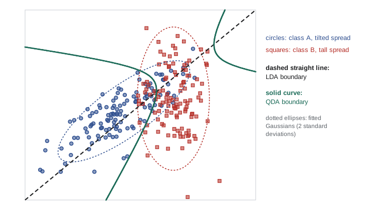
# Gaussian naive Bayes, LDA, QDA and logistic regression on data with unequal class covariances.
import numpy as np
from sklearn.naive_bayes import GaussianNB
from sklearn.discriminant_analysis import LinearDiscriminantAnalysis, QuadraticDiscriminantAnalysis
from sklearn.linear_model import LogisticRegression
rng = np.random.default_rng(367)
def make(n):
    a = rng.multivariate_normal([0, 0], [[1.0, 0.8], [0.8, 1.0]], n)      # correlated features
    b = rng.multivariate_normal([1.5, 0.5], [[0.3, 0.0], [0.0, 2.0]], n)  # a different shape
    return np.vstack([a, b]), np.r_[np.zeros(n), np.ones(n)]
Xtr, ytr = make(150); Xte, yte = make(5000)
for name, m in [("Gaussian naive Bayes", GaussianNB()), ("LDA (shared covariance)", LinearDiscriminantAnalysis()),
                ("QDA (separate covariances)", QuadraticDiscriminantAnalysis()),
                ("logistic regression", LogisticRegression())]:
    m.fit(Xtr, ytr)
    print(f"{name:27} test error {1 - m.score(Xte, yte):.3f}")

Gaussian naive Bayes        test error 0.150
LDA (shared covariance)     test error 0.153
QDA (separate covariances)  test error 0.131
logistic regression         test error 0.154

In this invented problem the two classes have very different covariance structures, so the true Bayes boundary is curved and QDA, whose assumptions match, wins clearly. LDA and logistic regression are both linear and perform similarly. Gaussian naive Bayes models each class with an axis-aligned ellipse; it can still draw a curved boundary, but it cannot represent the tilt of the first class, and it lands between the linear methods and QDA.

Generative versus discriminative

LDA and logistic regression produce the same form of classifier: a linear boundary, and posterior log odds that are linear in x. Indeed, if the LDA assumptions hold, the posterior is exactly a logistic function. The difference lies in how the weights are estimated. LDA fits the full joint distribution of x and y; logistic regression fits only the conditional distribution of y given x. When the Gaussian assumptions are true, LDA is more efficient, needing fewer examples for the same accuracy. When they are false, logistic regression is more robust, because it makes no claim about how x is distributed.

Andrew Ng and Michael Jordan made this trade-off precise in a 2002 paper comparing naive Bayes with logistic regression. The generative classifier approaches its (higher) asymptotic error quickly, needing a number of examples logarithmic in the number of features, while the discriminative classifier approaches its (lower) asymptotic error more slowly, needing a number linear in the features. So with little data, naive Bayes often wins; with plenty, logistic regression catches up and passes it. The program below reproduces the effect on invented binary data with 50 features, two of which are copied twice more, so that naive Bayes counts their evidence three times over: a sharp violation of the independence assumption.

# Generative versus discriminative: naive Bayes and logistic regression as training data grow.
import numpy as np
from sklearn.naive_bayes import BernoulliNB
from sklearn.linear_model import LogisticRegression
rng = np.random.default_rng(1)
d = 50
p1 = rng.uniform(0.2, 0.8, d); p0 = np.clip(p1 + rng.normal(0, 0.15, d), 0.05, 0.95)
p0[:2] = np.clip(p1[:2] + 0.2, 0.05, 0.95)
def make(n):
    y = rng.integers(0, 2, n)
    X = (rng.uniform(size=(n, d)) < np.where(y[:, None] == 1, p1, p0)).astype(int)
    return np.hstack([X, X[:, :2], X[:, :2]]), y     # two features appear three times each
Xte, yte = make(20000)
print("    n   naive Bayes error   logistic regression error")
for n in (10, 30, 100, 1000, 5000):
    e_nb, e_lr = [], []
    for rep in range(20):
        X, y = make(n)
        if len(set(y)) < 2: continue                   # need both classes to fit
        e_nb.append(1 - BernoulliNB().fit(X, y).score(Xte, yte))
        e_lr.append(1 - LogisticRegression(C=1.0, max_iter=2000).fit(X, y).score(Xte, yte))
    print(f"{n:5}   {np.mean(e_nb):17.3f}   {np.mean(e_lr):25.3f}")

    n   naive Bayes error   logistic regression error
   10               0.362                       0.416
   30               0.265                       0.287
  100               0.205                       0.230
 1000               0.174                       0.161
 5000               0.171                       0.153

Naive Bayes is ahead with 10, 30 and 100 training examples. By 1,000 examples logistic regression has overtaken it, and the gap persists at 5,000: naive Bayes keeps triple-counting the duplicated features, a bias that no amount of data removes, while logistic regression simply learns smaller weights for the copies. Which family to prefer therefore depends on how much labelled data you have, one more reason to compare candidates on validation data rather than by reputation.

Decision theory with probabilities

A probabilistic classifier separates two questions that a hard classifier merges: what is likely, and what should be done. Given posterior probabilities and a loss matrix \(L_{jk}\), the cost of predicting class k when the truth is j, the Bayes decision rule chooses the action with the smallest expected loss \(\sum_j L_{jk} P(y = j \mid \mathbf{x})\). With 0-1 loss this is the most probable class. If missing a fraudulent transaction costs 50 times as much as a false alarm, the rule flags a transaction whenever its fraud probability exceeds 1/51, about 2 per cent, rather than 50 per cent. Priors can also be adjusted at deployment time: if a spam filter was trained when half of all mail was spam and spam now makes up 80 per cent, the posteriors can be corrected by reweighting the prior without retraining the class-conditional models. These manipulations require probabilities that mean what they say, which is the subject of calibration in lesson 9.

Worked examples