Unsupervised learning: clustering and mixture models

Most data have no labels. A retailer has millions of transactions but no list of customer types; an astronomer has spectra of millions of stars but no catalogue of their classes; a hospital has years of sensor readings but no annotation of what each pattern means. Unsupervised learning looks for structure in such data without a target to predict. Clustering, the subject of this lesson, partitions examples into groups whose members are similar to each other and different from members of other groups. Dimensionality reduction, the subject of lesson 12, finds a small number of directions that capture most of the variation. Both are used to explore data, to compress it, to create features for supervised models, and to detect anomalies.

Unsupervised learning is harder to evaluate than supervised learning, because there is no ground truth to compare against. A clustering is useful if it helps someone understand or act on the data, and different clusterings of the same data can all be legitimate. This lesson develops the main methods, k-means, Gaussian mixture models with the EM algorithm, hierarchical clustering and density-based clustering, together with the assumptions each makes about what a cluster is, because choosing a method is choosing a definition.

k-means

k-means represents each of k clusters by a centre \(\boldsymbol{\mu}_j\) and assigns every point to its nearest centre. It seeks the centres and assignments that minimize the within-cluster sum of squared distances, called the inertia or distortion:

where c(i) is the cluster of point i. Finding the global minimum is NP-hard, but Lloyd's algorithm, devised by Stuart Lloyd at Bell Labs in 1957 and published in 1982, finds a local minimum by alternating two steps. In the assignment step, assign each point to the nearest centre. In the update step, move each centre to the mean of its assigned points. Each step can only decrease J: the assignment step chooses the best cluster for each point given the centres, and the update step chooses the best centre for each cluster given the assignments, since the mean minimizes the sum of squared distances. J is bounded below and there are finitely many assignments, so the algorithm converges, usually in a few dozen iterations.

It converges to a local minimum that depends on the starting centres, sometimes a poor one in which two centres share one true cluster while another pair of clusters is merged. The standard remedy is k-means++ seeding (David Arthur and Sergei Vassilvitskii, 2007): choose the first centre at random from the data, then choose each further centre with probability proportional to its squared distance from the nearest centre already chosen. This spreads the initial centres out, and it guarantees an expected inertia within a factor of \(O(\log k)\) of the optimum. In practice one also runs the algorithm several times from different seeds and keeps the best result.

# k-means (Lloyd's algorithm) with k-means++ seeding, written from scratch.
import numpy as np
rng = np.random.default_rng(367)
means_true = np.array([[0, 0], [4, 0], [2, 3.5], [6, 4]])
X = np.vstack([rng.normal(c, 0.7, (75, 2)) for c in means_true])

def kmeans_pp(X, k):
    C = [X[rng.integers(len(X))]]
    for _ in range(k - 1):
        d2 = np.min(((X[:, None] - np.array(C)[None]) ** 2).sum(axis=2), axis=1)
        C.append(X[rng.choice(len(X), p=d2 / d2.sum())])   # far points are more likely to be chosen
    return np.array(C)

def kmeans(X, k, iters=100):
    C = kmeans_pp(X, k)
    for it in range(iters):
        labels = ((X[:, None] - C[None]) ** 2).sum(axis=2).argmin(axis=1)   # assignment step
        newC = np.array([X[labels == j].mean(axis=0) for j in range(k)])     # update step
        if np.allclose(newC, C): break
        C = newC
    inertia = ((X - C[labels]) ** 2).sum()
    return C, labels, inertia, it + 1

def silhouette(X, labels):
    D = np.sqrt(((X[:, None] - X[None]) ** 2).sum(axis=2)); s = []
    for i in range(len(X)):
        same = labels == labels[i]; same[i] = False
        a = D[i, same].mean()
        b = min(D[i, labels == j].mean() for j in set(labels) if j != labels[i])
        s.append((b - a) / max(a, b))
    return np.mean(s)

print(" k   inertia   silhouette   iterations")
for k in (2, 3, 4, 5, 6, 8):
    C, lab, inertia, its = kmeans(X, k)
    print(f"{k:2}  {inertia:8.1f}   {silhouette(X, lab):10.3f}   {its:10}")
C, lab, _, _ = kmeans(X, 4)
print("cluster means found for k = 4:", np.round(C[np.argsort(C[:, 0] + 10 * C[:, 1])], 2).tolist())

 k   inertia   silhouette   iterations
 2    1465.7        0.447           15
 3     811.7        0.529            4
 4     259.0        0.685            3
 5     236.5        0.580           10
 6     207.7        0.505            5
 8     177.9        0.396           10
cluster means found for k = 4: [[0.11, 0.0], [3.99, 0.04], [1.99, 3.62], [6.01, 3.94]]

Choosing k

Inertia always decreases as k increases, reaching zero when every point is its own cluster, so it cannot choose k by itself. The elbow method plots inertia against k and looks for the point where adding clusters stops helping much; the elbow is often ambiguous. The silhouette coefficient compares, for each point, its mean distance a to other members of its cluster with its mean distance b to members of the nearest other cluster: \(s = (b - a)/\max(a, b)\), between −1 and 1. A high average silhouette means compact, well-separated clusters. In the run above the silhouette is highest at the k used to generate the data. Other criteria include the gap statistic and, for mixture models, information criteria such as BIC. Often the best answer comes from the application: a marketing team may want five segments because it can design five campaigns.

What k-means assumes

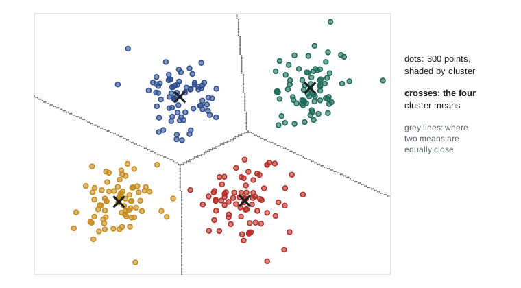
Because each point goes to its nearest centre, the boundaries between k-means clusters are straight lines (hyperplanes) and each cluster is a convex region. Because the objective is squared Euclidean distance, k-means favours roughly spherical clusters of similar size and spread, is sensitive to feature scaling, and is pulled around by outliers. It cannot find elongated, curved or nested clusters. Variants relax some assumptions: k-medoids uses actual data points as centres and any distance; mini-batch k-means scales to very large data; kernel k-means works in a feature space. When clusters differ in shape and size, a probabilistic model is a better fit.

Gaussian mixture models

A Gaussian mixture model (GMM) assumes each point was generated by first choosing a component k with probability \(\pi_k\), then drawing from a Gaussian with mean \(\boldsymbol{\mu}_k\) and covariance \(\Sigma_k\). The density of the data is

This is the generative model of lesson 8 with the class label unobserved, a latent variable. Instead of a hard assignment, a GMM gives each point a responsibility \(r_{ik} = P(z_i = k \mid \mathbf{x}_i)\), the posterior probability that it came from component k. Clusters can be elliptical, tilted and of different sizes, and points between clusters are honestly uncertain. A GMM is also a density estimate, which can flag anomalies as points of low density.

The EM algorithm

Maximizing the likelihood of a mixture directly is awkward, because the logarithm of a sum does not simplify. The expectation–maximization (EM) algorithm of Arthur Dempster, Nan Laird and Donald Rubin (1977) alternates two easy steps. In the E step, compute the responsibilities using the current parameters and Bayes' rule. In the M step, re-estimate each component's weight, mean and covariance as weighted averages, weighting each point by its responsibility:

Each iteration never decreases the likelihood, and the algorithm converges to a local maximum. k-means is a limiting case of EM for a GMM with equal spherical covariances shrinking to zero, in which responsibilities become hard 0-or-1 assignments. AI-320's lesson on latent variables derives EM in general, as coordinate ascent on a lower bound of the log-likelihood, and applies it to other models such as hidden Markov models.

# A Gaussian mixture model fitted by EM, from scratch, in one dimension.
import numpy as np
rng = np.random.default_rng(2)
# invented data: commute times (minutes) from two groups, transit riders and drivers
x = np.r_[rng.normal(42, 8, 300), rng.normal(22, 5, 200)]

def normal_pdf(x, mu, sd):
    return np.exp(-0.5 * ((x - mu) / sd) ** 2) / (sd * np.sqrt(2 * np.pi))

pi, mu, sd = np.array([0.5, 0.5]), np.array([15.0, 60.0]), np.array([10.0, 10.0])   # a poor start
for it in range(1, 201):
    # E step: responsibility of each component for each point
    dens = pi * np.column_stack([normal_pdf(x, mu[k], sd[k]) for k in range(2)])
    r = dens / dens.sum(axis=1, keepdims=True)
    loglik = np.log(dens.sum(axis=1)).sum()
    # M step: weighted maximum likelihood estimates
    Nk = r.sum(axis=0)
    pi, mu = Nk / len(x), (r * x[:, None]).sum(axis=0) / Nk
    sd = np.sqrt((r * (x[:, None] - mu) ** 2).sum(axis=0) / Nk)
    if it in (1, 2, 5, 20, 200):
        print(f"iteration {it:3}: log-likelihood {loglik:9.2f}  weights {np.round(pi, 3)}  means {np.round(mu, 2)}  sds {np.round(sd, 2)}")
print(f"P(transit group | 30 minutes) = {r[np.argmin(np.abs(x - 30)), np.argmax(mu)]:.2f} (for the observation nearest 30)")

iteration   1: log-likelihood  -2371.32  weights [0.595 0.405]  means [25.61 45.45]  sds [7.47 6.32]
iteration   2: log-likelihood  -1926.34  weights [0.584 0.416]  means [25.43 45.14]  sds [7.45 6.47]
iteration   5: log-likelihood  -1923.60  weights [0.553 0.447]  means [24.83 44.56]  sds [7.09 6.72]
iteration  20: log-likelihood  -1913.71  weights [0.437 0.563]  means [22.35 42.38]  sds [5.31 7.67]
iteration 200: log-likelihood  -1912.05  weights [0.383 0.617]  means [21.45 41.2 ]  sds [4.72 8.4 ]
P(transit group | 30 minutes) = 0.65 (for the observation nearest 30)

From a deliberately poor start, EM moves the components toward the two groups within a few iterations and then refines them slowly, with the log-likelihood rising at every step. The recovered weights, means and standard deviations are close to the values used to generate the data (60 per cent transit riders averaging 42 minutes, 40 per cent drivers averaging 22). A 30-minute commute is ambiguous, and the model says so with a responsibility between the extremes rather than forcing a choice.

GMMs have pitfalls of their own. A component can collapse onto a single point, its variance shrinking toward zero and its likelihood growing without bound; implementations guard against this by adding a small constant to the covariance diagonal or by placing priors on the parameters. Full covariance matrices have many parameters in high dimensions, so diagonal or tied covariances are common simplifications. And like k-means, EM finds local optima, so multiple restarts, often initialized from k-means, are standard.

Hierarchical clustering

Hierarchical clustering builds a tree of nested clusters rather than a single partition. Agglomerative clustering starts with every point as its own cluster and repeatedly merges the two closest clusters until one remains. The result is drawn as a dendrogram, whose merge heights show how far apart the merged clusters were; cutting the dendrogram at a chosen height gives a partition, and the tree shows the structure at every scale at once, which is valuable for exploration and is the norm in fields such as phylogenetics and gene-expression analysis.

The definition of distance between clusters, the linkage, determines the result. Single linkage uses the closest pair of points and can follow long, thin chains, finding elongated clusters but also chaining distinct clusters together through a few intermediate points. Complete linkage uses the farthest pair and produces compact clusters. Average linkage uses the mean pairwise distance. Ward's method merges the pair that least increases total within-cluster variance, giving results similar to k-means. Naive agglomerative clustering costs \(O(n^2)\) memory and at least \(O(n^2)\) time, so it suits thousands of points, not millions.

Density-based clustering

DBSCAN (Martin Ester, Hans-Peter Kriegel, Jörg Sander and Xiaowei Xu, 1996) defines clusters as dense regions separated by sparse ones. A point is a core point if at least min_samples points lie within distance eps of it. Clusters grow by connecting core points that are within eps of each other, together with the border points near them; points that belong to no cluster are labelled noise. DBSCAN finds clusters of arbitrary shape, determines their number automatically, and identifies outliers explicitly. It struggles when clusters have very different densities, which HDBSCAN addresses by considering all density levels, and its parameters must be chosen with the scale of the data in mind.

# k-means, single and Ward linkage, and DBSCAN on two interleaved half-moons.
import numpy as np
from sklearn.cluster import KMeans, AgglomerativeClustering, DBSCAN
from sklearn.metrics import adjusted_rand_score
rng = np.random.default_rng(0)
a = rng.uniform(0, np.pi, 200)
X = np.vstack([np.column_stack([np.cos(a[:100]), np.sin(a[:100])]),
               np.column_stack([1 - np.cos(a[100:]), 0.5 - np.sin(a[100:])])]) + rng.normal(0, 0.06, (200, 2))
truth = np.repeat([0, 1], 100)
models = {"k-means (k=2)": KMeans(2, n_init=10, random_state=0),
          "agglomerative, Ward": AgglomerativeClustering(2, linkage="ward"),
          "agglomerative, single link": AgglomerativeClustering(2, linkage="single"),
          "DBSCAN (eps=0.2, min_samples=5)": DBSCAN(eps=0.2, min_samples=5)}
for name, m in models.items():
    lab = m.fit_predict(X)
    extra = f"  clusters found {len(set(lab) - {-1})}, noise points {np.sum(lab == -1)}" if "DBSCAN" in name else ""
    print(f"{name:32} adjusted Rand index {adjusted_rand_score(truth, lab):6.3f}{extra}")

k-means (k=2)                    adjusted Rand index  0.288
agglomerative, Ward              adjusted Rand index  0.420
agglomerative, single link       adjusted Rand index  1.000
DBSCAN (eps=0.2, min_samples=5)  adjusted Rand index  1.000  clusters found 2, noise points 0

The adjusted Rand index (ARI) measures agreement between a clustering and a reference labelling, corrected for chance: 1 means perfect agreement, 0 means no better than random. Here the reference is the moon each point was generated from, available only because the data are invented. k-means and Ward linkage cut the moons with a straight boundary and score poorly, because they assume compact clusters. Single linkage and DBSCAN follow the curved shapes. With real data no reference exists, which is why internal measures such as the silhouette, stability under resampling and above all usefulness to the people who will act on the clusters are what count.

Clustering in practice

A few practical habits apply to all methods. Scale features first, since every method depends on distances or variances. Remember that a clustering algorithm will always return clusters, even from data with no structure at all; check stability by rerunning on bootstrap samples or subsets, and compare against clusterings of shuffled data. Interpret clusters by describing them (feature means, typical examples) and validate them against external information where possible. Beware of treating clusters as natural kinds: segmenting customers or patients into groups can be useful, but clusters found in data reflect the features chosen and the method used as much as any underlying reality, and decisions applied to whole clusters can treat individuals unfairly.

Worked examples