The learning problem

Machine learning is the study of programs that improve at a task through experience rather than through explicit instructions. A spam filter is not written as a list of rules about suspicious words; it is fitted to thousands of messages that people have already labelled. A model that predicts tomorrow's electricity demand is not derived from first principles; it is estimated from years of past demand and weather. This course develops the core methods of classical machine learning from a computing science point of view: how the algorithms work, why they work, when they fail, and how to tell the difference between a model that has learned something and one that has merely memorized its data.

Tom Mitchell's 1997 definition is still the clearest starting point: a program learns from experience E with respect to some class of tasks T and performance measure P if its performance at tasks in T, as measured by P, improves with experience E. Every learning problem in this course can be described by naming those three things. For spam filtering, T is classifying messages, P is the fraction classified correctly (or, better, a cost-weighted error), and E is a corpus of labelled messages. The definition forces a designer to say what improvement means before any code is written, which is the habit that separates machine learning engineering from curve fitting.

Where this course fits

CMPUT-366 surveyed artificial intelligence as search, logic, probability and planning, and its lesson on probabilistic reasoning introduced the Bayesian networks that reappear here as generative classifiers. STAT-151 introduced simple and multiple regression from a statistician's point of view, with the emphasis on inference about coefficients; this course reuses that machinery but asks a different question, namely how well a fitted model predicts new cases. The AI program offers depth on several of our topics: AI-110 shows how to use scikit-learn as a tool, AI-210 develops the linear algebra, probability and learning theory in more mathematical detail, AI-310 treats optimization, AI-320 treats probabilistic models and AI-460 treats fairness and privacy. CMPUT-466 follows this course with deep learning: neural networks at scale, convolutional networks and transformers. We meet a small neural network only in the final lesson.

Throughout the course the algorithms are implemented from scratch in NumPy, usually in fewer than thirty lines, and run on invented, seeded datasets so that every number printed on the page can be reproduced. Where scikit-learn offers the same method, we sometimes check our implementation against it. The point is not to replace the libraries, which are faster and better tested than anything written in a lesson, but to make sure that when you call them you know what they compute.

Kinds of learning

In supervised learning the experience consists of examples \((x_i, y_i)\), each an input paired with the correct output. If the output is a real number, such as a price, a temperature or a travel time, the task is regression. If the output is one of a finite set of categories, such as spam or not spam, or one of ten digits, the task is classification; with two categories it is binary classification. Most of this course concerns supervised learning, because it is the best understood setting and the one where the ideas of generalization are sharpest.

In unsupervised learning the examples have no labels, and the goal is to discover structure: groups of similar cases (clustering), a small number of underlying directions that explain most of the variation (dimensionality reduction), or the shape of the distribution itself (density estimation). Lessons 11 and 12 cover these methods. Self-supervised learning, which powers modern language models, manufactures labels from the data itself, for example by hiding a word and asking the model to predict it; CMPUT-466 and AI-410 treat it. Reinforcement learning, in which an agent learns from rewards obtained by acting, is the subject of AI-330 and was previewed in CMPUT-366's lesson on Markov decision processes.

The formal setup

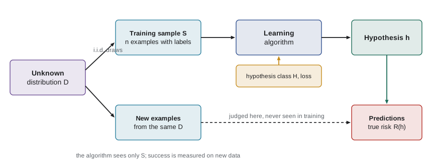
To reason about learning we need a precise model of what the data are and what success means. The standard model of supervised learning has five ingredients.

First, an input space \(\mathcal{X}\) and an output space \(\mathcal{Y}\). For a model that predicts whether a campus will close for snow, an input might be a vector of forecast snowfall, temperature and wind, so \(\mathcal{X} = \mathbb{R}^3\), and \(\mathcal{Y} = \{0, 1\}\).

Second, an unknown probability distribution \(\mathcal{D}\) over pairs \((x, y)\). The distribution captures both how inputs occur and how labels relate to inputs, including noise: two days with identical forecasts might end differently. We never know \(\mathcal{D}\); all we see is data drawn from it.

Third, a training sample \(S = ((x_1, y_1), \ldots, (x_n, y_n))\) whose examples are drawn independently from \(\mathcal{D}\). This is the i.i.d. assumption: independent and identically distributed. It is what lets performance on past data say anything about performance on future data, and it is the assumption most often violated in practice, for example when the world changes after deployment or when several examples come from the same patient, customer or sensor.

Fourth, a hypothesis class \(\mathcal{H}\), the set of functions \(h: \mathcal{X} \to \mathcal{Y}\) that the learning algorithm is allowed to output. Linear functions, decision trees of depth at most five and neural networks with a fixed architecture are all hypothesis classes. Choosing \(\mathcal{H}\) is the most consequential decision a practitioner makes, because no algorithm can return a function outside it.

Fifth, a loss function \(\ell(\hat{y}, y)\) that measures the cost of predicting \(\hat{y}\) when the truth is \(y\). The quantity we actually care about is the expected loss on a new example, called the true risk or generalization error:

Because \(\mathcal{D}\) is unknown, \(R(h)\) cannot be computed. What can be computed is the empirical risk, the average loss on the training sample:

Loss functions

Different tasks call for different losses. For regression, the squared loss \((\hat{y} - y)^2\) is the default: it is smooth, it leads to closed-form solutions for linear models, and minimizing its expectation gives the conditional mean \(\mathbb{E}[y \mid x]\). The absolute loss \(\lvert \hat{y} - y \rvert\) is less sensitive to outliers and is minimized by the conditional median. For classification, the natural measure is the 0-1 loss, which is 1 for a mistake and 0 otherwise; its expectation is the error rate. The 0-1 loss is discontinuous and hard to optimize directly, so classifiers are usually trained on a smooth surrogate such as the logistic (cross-entropy) loss of lesson 4 or the hinge loss of lesson 5, and evaluated with 0-1 loss or the richer measures of lesson 9.

The last column matters. A loss is a statement of what you want. If a hospital cares about missing a disease far more than about a false alarm, then the symmetric 0-1 loss is the wrong loss, and the best classifier under the right one will flag more patients. Lesson 9 returns to cost-sensitive decisions and threshold choice.

The classifier that minimizes expected 0-1 loss, predicting for each x the most probable label under \(\mathcal{D}\), is called the Bayes classifier, and its risk is the Bayes error. The Bayes error is the irreducible floor set by noise in the labels: no learner, however clever, can beat it. On the invented snow data below, even the best threshold rule is wrong on roughly one day in eleven, because closures are only partly predictable from snowfall.

Empirical risk minimization

The simplest learning principle is empirical risk minimization (ERM): choose the hypothesis in \(\mathcal{H}\) with the smallest training error,

ERM is behind ordinary least squares, behind most decision tree and neural network training, and behind many methods that add a penalty to the empirical risk. The central question of learning theory is when ERM works, that is, when a small empirical risk implies a small true risk. The program below runs ERM on a tiny hypothesis class: threshold rules that predict a campus closure whenever forecast snowfall exceeds t centimetres, for t from 0 to 40. A very large sample from the same invented distribution stands in for the true risk.

# Empirical risk minimization over a finite class of threshold rules.
# Invented data: x = overnight snowfall forecast (cm), y = 1 if the campus closed.
import numpy as np
rng = np.random.default_rng(367)

def draw(n):
    x = rng.uniform(0, 40, n)
    p = 1 / (1 + np.exp(-(x - 22) / 2.5))   # the unknown "true" relationship
    y = (rng.uniform(size=n) < p).astype(int)
    return x, y

thresholds = np.arange(0, 41)               # H = {h_t(x) = 1 if x >= t}, 41 hypotheses
def risk(t, x, y):
    return np.mean((x >= t).astype(int) != y)   # 0-1 loss, averaged

x_big, y_big = draw(200_000)                # a huge sample stands in for the true distribution
true_risk = np.array([risk(t, x_big, y_big) for t in thresholds])
print(f"best possible threshold in H: t = {thresholds[true_risk.argmin()]}, true risk {true_risk.min():.3f}")
for n in (10, 30, 100, 1000):
    x, y = draw(n)
    emp = np.array([risk(t, x, y) for t in thresholds])
    t_hat = thresholds[emp.argmin()]        # ERM: pick the rule with the smallest training error
    print(f"n = {n:4}: ERM picks t = {t_hat:2}, empirical risk {emp.min():.3f}, true risk {true_risk[t_hat]:.3f}")

best possible threshold in H: t = 22, true risk 0.086
n =   10: ERM picks t = 14, empirical risk 0.200, true risk 0.204
n =   30: ERM picks t = 16, empirical risk 0.200, true risk 0.160
n =  100: ERM picks t = 23, empirical risk 0.110, true risk 0.089
n = 1000: ERM picks t = 23, empirical risk 0.091, true risk 0.089

With 10 or 30 examples, ERM picks a threshold far from the best one, and its true risk is roughly twice the best achievable: a small sample can make a poor rule look as good as any other. As n grows, the empirical risk of the chosen rule moves toward its true risk, and the chosen threshold moves toward the best one in the class. This convergence is not an accident; lesson 2 proves that for a finite class like this one, the gap shrinks at a rate proportional to \(\sqrt{\log \lvert \mathcal{H} \rvert / n}\).

Generalization and the danger of memorizing

Minimizing training error is necessary but not sufficient. A hypothesis class rich enough to fit any training set perfectly will fit the noise as well as the signal. The extreme case is a lookup table: memorize every training example, answer with its label, and guess for anything new. Training error is zero. Whether it has learned anything depends entirely on whether the test inputs repeat the training inputs, and in any interesting problem they do not.

# A memorizer versus a simple rule: zero training error is not the goal.
import numpy as np
rng = np.random.default_rng(1)
n_train, n_test = 200, 5000
def sample(n):
    X = rng.integers(0, 2, size=(n, 20))      # 20 yes/no features, about a million possible inputs
    noise = rng.uniform(size=n) < 0.10        # 10% of labels are flipped
    y = (X[:, 0] ^ noise).astype(int)         # the label really depends only on feature 0
    return X, y
Xtr, ytr = sample(n_train); Xte, yte = sample(n_test)

table = {tuple(r): t for r, t in zip(Xtr, ytr)}  # memorizer: look the input up, else guess 0
memo = lambda X: np.array([table.get(tuple(r), 0) for r in X])
rule = lambda X: X[:, 0]                         # a one-feature rule
for name, h in [("memorizer", memo), ("one-feature rule", rule)]:
    print(f"{name:17} training error {np.mean(h(Xtr) != ytr):.3f}   test error {np.mean(h(Xte) != yte):.3f}")
seen = np.mean([tuple(r) in table for r in Xte])
print(f"fraction of test inputs seen during training: {seen:.4f}")

memorizer         training error 0.000   test error 0.505
one-feature rule  training error 0.105   test error 0.099
fraction of test inputs seen during training: 0.0000

The memorizer has zero training error and roughly chance test error, because almost none of the 5,000 test inputs appeared in training. The one-feature rule makes about 10 per cent errors on both sets, which is the noise rate we built into the data, so it is close to the Bayes classifier. The difference between training error and test error is called the generalization gap. Machine learning is, in large part, the art of keeping that gap small while also keeping the training error small.

Training, validation and test data

Because the true risk cannot be computed, we estimate it with held-out data. The standard protocol splits the available labelled data into three parts. The training set is used to fit model parameters. The validation set (sometimes called the development set) is used to make choices about the model: which hypothesis class, which regularization strength, which features, when to stop training. The test set is used once, at the end, to estimate the performance of the final model on new data.

The discipline lies in that word once. Every time a decision is made by looking at a data set, that data set becomes part of the training process, and its error becomes an optimistic estimate. A team that evaluates fifty model variants on the test set and reports the best has, in effect, trained on the test set. Lesson 9 develops cross-validation, which reuses limited data more efficiently, and nested cross-validation, which keeps model selection honest. Lesson 10 treats data leakage, the broader family of ways in which information about the test set sneaks into training.

Typical split proportions are 60/20/20 or 70/15/15 for moderate data sets; with millions of examples, a test set of a few thousand may be enough, since the standard error of an error-rate estimate p from m test cases is about \(\sqrt{p(1-p)/m}\). With 2,000 test cases and a true error near 10 per cent, the standard error is about 0.7 percentage points, so differences between models smaller than about 1.5 points cannot be distinguished reliably from that test set alone.

Inductive bias

A learner must prefer some hypotheses to others before seeing the data, or it cannot generalize at all. That built-in preference is its inductive bias. A linear regression assumes that the output changes linearly with each input. A k-nearest-neighbour classifier assumes that nearby inputs have similar labels. A decision tree prefers axis-aligned splits and, when grown greedily, short trees. A convolutional network assumes that the same local pattern means the same thing wherever it appears in an image. Inductive bias comes from two sources: the restriction to a hypothesis class, and the preferences within the class expressed by regularization, priors or the search procedure.

Inductive bias is not a flaw to be eliminated. The memorizer above has almost no bias in the relevant sense, which is exactly why it fails. The aim is a bias that matches the problem: strong enough to rule out the noise-fitting hypotheses that the data cannot rule out, weak enough to contain a hypothesis close to the truth. Much of the progress in machine learning has come from finding biases that suit particular kinds of data, such as images, sequences and graphs.

No free lunch

The no free lunch theorems, proved by David Wolpert and William Macready in the 1990s, make the role of bias precise. Averaged over all possible target functions on a finite input space, every learning algorithm has the same expected error on inputs it has not seen. For any algorithm that does well on some problems, there are equally many problems on which it does badly. A learner that predicts the opposite of the training labels does exactly as well, averaged over every possible world, as one that predicts the training labels.

The theorem does not say that all algorithms are equally good in practice. It says that an algorithm's advantage must come from assumptions about which problems are likely, and the real world is not a uniform average over all functions: nearby houses do have similar prices, and the labels of images do not change when an object shifts by one pixel. The practical lesson is that there is no universally best classifier. Comparing several hypothesis classes on validation data, as lesson 9 describes, is not indecision; it is the only honest way to find out which assumptions suit a problem.

A learning project from start to finish

A realistic machine learning project rarely starts with an algorithm. It starts with a decision someone needs to make, and works backward to data and models. The stages are roughly these. Frame the problem: what will the prediction be used for, what does an error cost, and what simple baseline (always predict the most common class, predict yesterday's value) must the model beat? Collect and understand the data: where it came from, what population it represents, how labels were assigned, and what could leak information from the future. Prepare features: clean, encode and scale, as lesson 10 describes. Choose candidate hypothesis classes and fit them, using validation data to tune them. Evaluate the final choice once on test data, with appropriate uncertainty. Deploy and monitor, since the distribution will drift.

Most failures in practice come from the first two stages, not from the choice between a support vector machine and a random forest. A model trained on images of skin lesions taken in a specialist clinic may fail on photographs from a phone; a fraud model trained before a new payment method launched may miss the fraud that method attracts. Keep the formal setup in mind: everything rests on the assumption that the training data and the future data come from the same distribution \(\mathcal{D}\). When that assumption is false, the guarantees in this course do not apply.

Worked examples