Soft processors, SoC FPGAs and HLS overview

Few FPGA designs are pure hardware. Most contain a processor somewhere, either built from the fabric as a soft core or present as hard silicon on the same chip, because sequential decisions, protocol stacks, configuration and anything that changes often are easier to write in software. This lesson covers how processors and programmable logic are combined: soft processors, SoC FPGAs with hard processor subsystems, the memory-mapped registers, interrupts and DMA that connect software to hardware, and how to decide which functions belong where. It ends with high-level synthesis (HLS), which generates hardware from C or C++ and changes how some of this work is done.

For the NS-5 revision B, Ines and Maren had three options. They could keep the existing microcontroller and add a separate FPGA beside it, joined by a fast serial link. They could use an FPGA alone, with a soft processor in the fabric running the firmware. Or they could use an SoC FPGA, a single chip with a hard processor subsystem and programmable logic. This lesson works through the trade-offs that led them to the third.

Soft processors

A soft processor is a processor described in RTL and synthesized into the fabric like any other block. Small 32-bit RISC-V cores, many of them open source, take from under a thousand to a few thousand LUTs, a few block RAMs for instruction and data memory, and run at 100 to 300 MHz in mid-range devices. Larger soft cores with caches, memory management and floating point take tens of thousands of LUTs. The attractions are flexibility and portability: the core can be configured with exactly the features needed, extended with custom instructions that call hardware accelerators, and moved to a different FPGA family with the rest of the design.

Soft processors are slower than hard processors by an order of magnitude and use fabric that could do other work. They suit control-plane tasks: sequencing hardware blocks, parsing commands, running a small network stack or a bootloader, reporting status. In a design like the NS-5 Lite, a single-channel low-cost variant, a small soft RISC-V core could replace the microcontroller entirely. In the full NS-5, the firmware from CMP-440, with its real-time kernel, classifier and CAN stack, needs more processing than a soft core provides.

SoC FPGAs

An SoC FPGA combines a hard processor subsystem with programmable logic on one die. The processor subsystem typically contains one or more application-class cores, sometimes a separate real-time core, caches, a DDR memory controller, and standard peripherals such as Ethernet, USB, CAN, SPI and UART. It boots and runs like any embedded processor, and it can configure the programmable logic, at power-up or later. The programmable logic is connected to the processor subsystem through several on-chip bus interfaces, usually following AXI conventions: some in which the processor is the master, for accessing registers in the fabric, and some in which the fabric is the master, for DMA into the processor's memory.

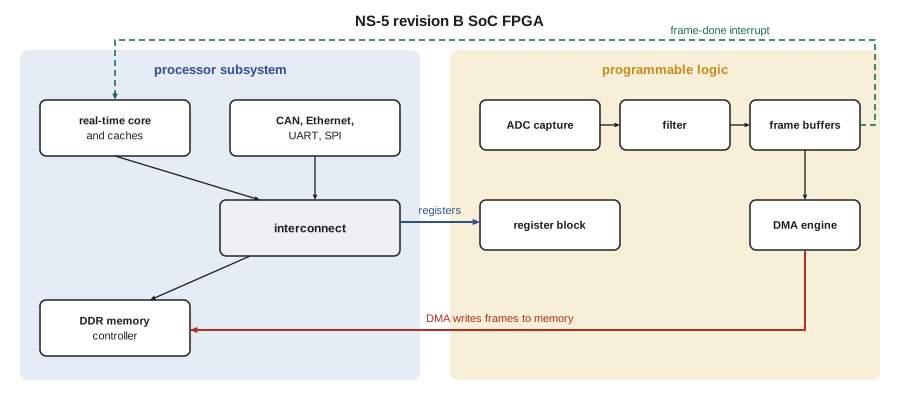
For the NS-5, the SoC FPGA won on board space, power and simplicity: one chip replaces two, the processor and front end share one memory, and the link between them is an on-chip bus rather than a board-level serial interface with its own timing and signal integrity concerns. The processor subsystem's real-time core runs the existing firmware, rebuilt for a new target, and the front end of lessons 6 to 10 lives in the programmable logic.

Connecting software to hardware

Three mechanisms connect the processor to logic in the fabric. Memory-mapped registers give software control and status: the front end has a small block of 32-bit registers at a base address, for start and abort bits, the gain and offset settings, frame counters, overflow flags and the peak FIFO occupancy. The processor reads and writes them with ordinary load and store instructions through a lightweight register-access bus.

// register block on a simple 32-bit register bus (address, write strobe, read data)
localparam logic [7:0] R_CTRL = 8'h00, R_STATUS = 8'h04, R_OFFSET = 8'h08,
                       R_FRAMES = 8'h0C, R_PEAK = 8'h10;

always_ff @(posedge clk) begin
    if (rst) begin
        abort <= 1'b0;  irq_en <= 1'b0;  done_flag <= 1'b0;
    end else begin
        start <= 1'b0;                                  // single-cycle pulse
        if (wr && addr == R_CTRL) begin
            start  <= wdata[0];
            abort  <= wdata[1];
            irq_en <= wdata[8];
        end
        if (wr && addr == R_OFFSET) offset <= wdata[11:0];
        if (wr && addr == R_STATUS && wdata[0]) done_flag <= 1'b0;   // write 1 to clear
        else if (done_evt)                        done_flag <= 1'b1;
    end
end

always_ff @(posedge clk)                                // registered read multiplexer
    unique case (addr)
        R_CTRL:   rdata <= {23'b0, irq_en, 6'b0, abort, 1'b0};
        R_STATUS: rdata <= {28'b0, fifo_ovf, busy, 1'b0, done_flag};
        R_OFFSET: rdata <= {20'b0, offset};
        R_FRAMES: rdata <= frame_count;
        R_PEAK:   rdata <= {23'b0, fifo_peak};
        default:  rdata <= 32'hDEAD_0BAD;               // makes bad addresses easy to spot
    endcase

assign irq = done_flag && irq_en;

Interrupts tell software that something happened without making it poll. The front end raises one interrupt line when a frame is complete; the handler reads the status register, clears the done flag by writing 1 to it, swaps the buffer pointers and wakes the radar task. The write-one-to-clear convention avoids a race in which software, reading and rewriting a whole status register, could accidentally clear a flag that hardware set in between.

Direct memory access moves bulk data without the processor. The front end's DMA engine takes the stream of filtered samples from its FIFO, packs them into bursts and writes each frame to a buffer in DDR memory whose address firmware has programmed. The processor never touches the samples until the frame is complete. This is where the 150 µs stall of lesson 7 comes from: the DMA competes for the memory controller with the processor and other masters. Caches add one more concern: the processor must not read stale cached copies of a buffer that the DMA has just written, so firmware either invalidates the cache lines for the buffer before reading it or maps the buffers as non-cacheable. Getting this wrong produces frames that are occasionally, and confusingly, a frame old.

Hardware and software partitioning

Deciding what goes in hardware is a quantitative question. A function belongs in hardware when it is regular, data-parallel, performed at a high rate and stable in its definition; it belongs in software when it is irregular, branchy, infrequent or likely to change. Filtering every sample is the textbook hardware function. Classification, which changes with every firmware release, stays in software. The calculation below estimates the cost of the filter in software on the SoC's real-time core and on a soft core, then the schedules a high-level synthesis tool would produce for several versions of the same C code, and finally the effect of the offload on the radar task as a whole.

from math import ceil

OUT_RATE = 4 * 500e3              # filtered outputs per second, all channels
MACS = 16                         # multiply-accumulates per output with the pre-adder

# 1. the filter as software
for name, f_cpu, cyc_per_mac in [("SoC real-time core, 400 MHz", 400e6, 1.6),
                                 ("soft RISC-V core, 100 MHz", 100e6, 3.0)]:
    load = OUT_RATE * (MACS * cyc_per_mac + 20) / f_cpu     # 20 cycles of loop overhead
    print(f"software filter on {name}: {100 * load:5.1f} % of the core")

# 2. the filter as high-level synthesis output: latency = (trip - 1) * II + depth
def hls(trip, ii, depth, f=100e6):
    lat = (trip - 1) * ii + depth
    return lat, 100 * OUT_RATE * lat / f

variants = [
    ("as written: one RAM port, 2 reads/iter", 16, 2, 6),
    ("history split into two banks", 16, 1, 6),
    ("float accumulator, add latency 4", 16, 4, 9),
    ("fully unrolled, partitioned arrays", 1, 1, 9),
]
print("HLS schedule for one output (100 MHz):")
for name, trip, ii, depth in variants:
    lat, load = hls(trip, ii, depth)
    print(f"  {name:40s} II={ii}  latency {lat:3d} cycles  engine load {load:5.1f} %")

# 3. Amdahl: what offloading the filter does for the whole radar task
f_filter = 0.85                   # share of the old radar task spent filtering
for speedup in (10, 100, float("inf")):
    s = 1 / ((1 - f_filter) + f_filter / speedup)
    print(f"filter {speedup:>5} x faster -> radar task {s:4.1f} x faster")

software filter on SoC real-time core, 400 MHz:  22.8 % of the core
software filter on soft RISC-V core, 100 MHz: 136.0 % of the core
HLS schedule for one output (100 MHz):
  as written: one RAM port, 2 reads/iter   II=2  latency  36 cycles  engine load  72.0 %
  history split into two banks             II=1  latency  21 cycles  engine load  42.0 %
  float accumulator, add latency 4         II=4  latency  69 cycles  engine load 138.0 %
  fully unrolled, partitioned arrays       II=1  latency   9 cycles  engine load  18.0 %
filter    10 x faster -> radar task  4.3 x faster
filter   100 x faster -> radar task  6.3 x faster
filter   inf x faster -> radar task  6.7 x faster

On the SoC's 400 MHz real-time core, the filter alone would take about 23 % of the processor, time that the classifier, now heavier with the pedestrian feature, needs. On a 100 MHz soft core it would take 136 %, more than the core has. In hardware, the MAC engine handles it at 36 % load of one DSP slice. The Amdahl calculation at the end makes a separate point: filtering was 85 % of the old radar task, so even infinitely fast filtering speeds the radar task up by at most 1 / 0.15, about 6.7 times. The remaining 15 %, frame bookkeeping and feature extraction, now dominates, and further gains must come from there.

High-level synthesis

High-level synthesis tools take a function written in C, C++ or a similar language, with directives that guide the hardware architecture, and generate RTL. They perform the scheduling, allocation and binding of lesson 5 automatically: they build a data-flow graph of the operations, assign each to a clock cycle given the target frequency and the delays of the device's operators, decide how many units to use, and generate a datapath and a controller. The key performance figures are the latency of a function or loop, the number of cycles from input to output, and the initiation interval (II), the number of cycles between starting successive iterations or calls.

// filter kernel for high-level synthesis; directives are written as comments
// here because their exact syntax differs between tools
#include <cstdint>
constexpr int N = 32, H = N / 2;

int32_t fir_out(const int16_t hist[64], int head, const int16_t coef[H]) {
    // directive: split hist into two banks so both samples of a pair are read in one cycle
    int64_t acc = 1 << 10;                       // rounding constant, as in lesson 6
    for (int k = 0; k < H; k++) {
        // directive: pipeline this loop with an initiation interval of 1
        int16_t a = hist[(head - k) & 63];
        int16_t b = hist[(head - (N - 1) + k) & 63];
        acc += int32_t(a + b) * coef[k];         // pre-add, multiply, accumulate
    }
    int64_t y = acc >> 11;
    return y > 32767 ? 32767 : y < -32768 ? -32768 : int32_t(y);   // saturate
}

For a pipelined loop, the latency is approximately:

where N_trip is the trip count and D the depth of one iteration's pipeline. The four variants in the code block show what limits II. As written, the history array maps to a memory with one read port, and each iteration needs two reads, so the tool cannot start an iteration every cycle: II = 2 and the latency is 36 cycles. Splitting the array into two banks, by an array-partitioning directive, gives two ports and II = 1, for 21 cycles. Accumulating in floating point instead would make II = 4, because each addition must wait for the previous one to finish its four-cycle pipeline, a loop-carried dependency. Fully unrolling the loop with partitioned arrays computes an output in 9 cycles but uses 16 multipliers.

These are exactly the trade-offs a hand designer makes, and HLS does not remove the need to understand them. What it changes is the cost of exploring them: a directive changes the architecture in minutes, where rewriting RTL takes days. HLS is widely used for signal and image processing kernels, linear algebra and machine-learning inference, and for algorithm developers who want hardware acceleration without writing RTL. It is less suited to control-dominated logic, precise interface timing and designs where every LUT matters. Its output must still be verified: the usual flow tests the C function against a reference in software, then runs a co-simulation that drives the generated RTL with the same test vectors, and finally includes the block in the full design's timing closure.

Jonah wrote the HLS version of the filter as an experiment and compared it with his hand-written RTL. With the two-bank directive, the generated design met 100 MHz with one DSP slice and about 20 % more LUTs than the hand-written version, and passed the bit-accurate vectors of lesson 6 at the first attempt. Ines kept the RTL for the product, because the team knows it and its timing is under direct control, but the HLS version is now the starting point for the next feature, a fast Fourier transform for velocity estimation.

Boot, configuration and software for the fabric

An SoC FPGA powers up its processor first, which runs a first-stage bootloader from flash, configures the programmable logic with the bitstream, and then starts the operating system or real-time kernel. Software therefore owns the order: the front end does not exist until the processor has loaded it, and drivers must wait for configuration to complete before touching its registers. A device description, generated from the hardware design, records the base address, interrupt number and register layout of each block in the fabric, so that the hardware and software teams work from one source of truth. At Northway Sensing, the register map is written once, in a machine-readable file, and both the RTL register block and the firmware header are generated from it, so the two cannot drift apart.