Digital system design flow and FPGA architecture: LUTs, CLBs, BRAM, DSP slices, routing

This course follows Northway Sensing, the Kingston, Ontario company whose roadside traffic sensors you met in earlier computer engineering courses, into the part of the product where software stops being fast enough. In CMP-440 the NS-5's radar task needed 1.2 ms of processor time every 6.25 ms, most of it spent filtering raw samples before the classifier ever saw them. The revision B board, now being designed for the Ontario Ministry of Transportation and City of Kingston pilot, adds two more receive antennas and doubles the sample rate. Doing that filtering in firmware would take more than the whole processor. Hardware lead Ines Carvalho's answer is to move the radar front end into a field-programmable gate array (FPGA), and she has asked Jonah Abara, in his final co-op term, to design it with her.

ELE-210 (cross-listed as CMP-210) ended with a first look at hardware description languages and programmable logic: a counter in Verilog, a seven-segment decoder, and the idea that a lookup table can implement any small Boolean function. This course starts where that lesson stopped. By lesson 12 you will have designed, verified and timed the complete NS-5 sensor front-end accelerator: a four-channel capture interface, a clock-domain crossing, a decimating fixed-point filter, frame buffers, a streaming interface into the processor's memory, configuration over SPI and a debug UART. Along the way you will learn to think about hardware the way synthesis tools and timing analyzers do, which is the real skill of digital system design.

This first lesson sets out the design flow that every FPGA project follows, then opens up the device itself. Knowing what the fabric contains, and what each resource costs, is what lets a designer write code that maps well and estimate a design's size before writing it.

Why an FPGA?

The NS-5 revision B front end must accept four channels of 12-bit samples at 2 million samples per second (MS/s) each, low-pass filter every channel with a 32-tap filter, reduce the rate by four, and deliver 1,024-sample frames to the processor. Counting multiply-accumulate operations (MACs) shows the size of the problem. A 32-tap filter computed at the full input rate needs 32 MACs per input sample, so four channels at 2 MS/s need 256 million MACs per second. Even computing only the outputs that survive decimation, 64 million MACs per second remain, plus the loads, stores and loop overhead around each one. The NS-5's microcontroller would spend all of its time on this and still fall behind.

There are three ways to get dedicated hardware. A custom chip, an application-specific integrated circuit (ASIC), gives the lowest unit cost and power at high volume, but its mask set and verification cost millions and a bug means a new chip. A digital signal processor or a faster application processor keeps everything in software but costs power and still processes samples one instruction at a time. An FPGA sits between them: a chip full of configurable logic, memory and arithmetic blocks connected by programmable routing, whose function is set by loading a configuration file called a bitstream. It can do many operations in parallel every clock cycle, it can be changed after the product ships, and it costs nothing extra to respin. The price is that the same function takes several times more silicon area and power than in an ASIC and runs at a lower clock rate, typically 100 to 500 MHz for a design rather than several gigahertz. For a product made in thousands rather than millions, with interfaces and algorithms that will change during a pilot, the FPGA is the clear choice.

The digital system design flow

An FPGA design passes through the same stages whether it is a 200-line interface block or a million-gate accelerator. The figure shows the flow and its feedback loops.

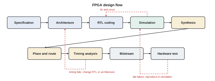
The specification states what the block must do in measurable terms: sample rates, latencies, interfaces, error behaviour, and the clock frequency and device it must fit. The architecture divides the function into blocks, chooses how much parallelism each needs and fixes the interfaces between them. This is where the biggest decisions are made, such as whether the filter uses 32 multipliers or one multiplier used 32 times.

Register-transfer level (RTL) coding describes each block as registers and the combinational logic between them, in Verilog, SystemVerilog or VHDL. Simulation runs the RTL against a testbench to show that it behaves as specified; lessons 4 and 12 treat verification in depth. Synthesis translates the RTL into a netlist of device primitives: lookup tables, flip-flops, carry chains, block memories and DSP slices. Implementation places each primitive at a physical site on the chip and routes the connections between them. Static timing analysis (STA) then checks that every path meets the clock constraints, as lesson 9 explains. Bitstream generation turns the placed and routed design into the configuration file, and hardware test loads it into a real board.

Two features of the flow surprise software engineers. The first is that simulation and synthesis interpret the same source code in different ways. A simulator executes the code; a synthesis tool infers hardware from it, and some constructs that simulate perfectly have no hardware meaning or produce hardware that behaves differently. Lessons 2 and 3 are largely about writing code that means the same thing to both. The second is that a design can be logically correct and still fail because it is too slow. Timing is a design requirement like any other, and the architecture must leave room to meet it.

Lookup tables

The basic logic element of an FPGA is the lookup table (LUT). A k-input LUT is a small memory of 2^k bits whose address lines are the k inputs. Configuring the LUT means writing its truth table into those bits, so a single LUT implements any Boolean function of its inputs, however complex, with the same delay. The number of distinct functions of k inputs is:

which is 16 for k = 2, 65,536 for k = 4 and about 1.8 × 10^19 for k = 6. Modern FPGAs use six-input LUTs, usually fracturable into two five-input LUTs that share inputs and produce two outputs. Synthesis cost is therefore measured in LUTs rather than gates: an expression of six variables costs one LUT whether it is an AND gate or a parity function, while a function of seven variables costs at least two.

LUTs also serve as small memories. Because a LUT is a memory, it can be written at run time, giving distributed RAM: a six-input LUT becomes a 64 × 1 synchronous-write, asynchronous-read RAM. Chained internally, the same LUT becomes a shift register of up to 32 bits without using any flip-flops, which is ideal for delay lines such as the sample history of a filter. Not every LUT in a device can do this; typically a quarter to a half of them can.

Logic blocks, carry chains and flip-flops

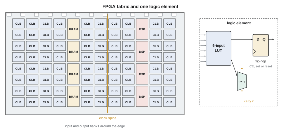
LUTs are grouped with flip-flops and arithmetic support into a configurable logic block (CLB), which different families divide into slices or logic elements. A typical CLB contains eight six-input LUTs, sixteen flip-flops, a dedicated carry chain and the wide multiplexers mentioned above, all with fast local connections. Each flip-flop has a clock enable and a set or reset input, and the flip-flops in a CLB share their clock and control signals, which is one reason that designs with many different enables or resets pack poorly.

The carry chain is the most important special structure. A ripple-carry adder built from general logic would need a LUT and a routing hop per bit for the carry. Instead, each LUT feeds a dedicated carry multiplexer and XOR gate, and the carry runs vertically through a hard-wired chain from one CLB to the next with a delay of a few tens of picoseconds per bit. A 32-bit adder therefore costs 32 LUTs and runs at several hundred megahertz. Synthesis uses the chain automatically for adders, subtractors, counters and comparators, provided the code describes them as arithmetic.

Block RAM

Larger memories use block RAM (BRAM), dedicated memory blocks arranged in columns across the die. A typical block holds 36 Kbit and can be split into two independent 18 Kbit blocks. Each block is a true dual-port memory: two independent ports, each with its own clock, address, data and write enable, so one port can be written in one clock domain while the other is read in another. The aspect ratio is configurable. A 36 Kbit block can be 32K × 1, 16K × 2, 8K × 4, 4K × 9, 2K × 18, 1K × 36 or, using both ports together, 512 × 72; the 9-bit multiples include a parity bit per byte.

Block RAM has one property that shapes how memories must be coded: the read is synchronous. The address is captured on a clock edge and the data appears after it, so a read takes at least one cycle, and two if the optional output register is used for speed. Code that expects data to appear in the same cycle as the address, which is natural in software, cannot map to block RAM and is built from LUTs instead, often at great cost. Lesson 7 covers memory inference in detail.

DSP slices

Multiplication is expensive in LUTs: an 18 × 18 multiplier built from logic takes roughly 300 LUTs and is slow. FPGAs therefore include hard DSP slices. A typical slice contains a pre-adder, a 25 × 18 signed multiplier, a 48-bit adder and accumulator, and pipeline registers at each stage, so a complete multiply-accumulate runs at over 400 MHz when all the internal registers are used. Slices are arranged in columns with dedicated cascade connections, so a chain of slices can form an adder tree or a systolic filter without using general routing. The NS-5 filter of lesson 6 is designed around one such slice.

Routing, clocks and input-output

The resources above occupy perhaps a fifth of the die. The rest is routing: wire segments of several lengths running horizontally and vertically between the blocks, joined by programmable switches in switch boxes. Each switch is a pass transistor or multiplexer controlled by a configuration bit, so every connection passes through several switches, and in a typical FPGA design half or more of each path's delay is in routing rather than logic. This is why the same logic can meet timing in one place-and-route run and miss it in another, and why designers think in terms of logic levels: the number of LUTs a signal passes through between two flip-flops.

Clocks are distributed separately on dedicated low-skew networks, typically a spine and branches reaching every flip-flop in a region, driven by global buffers. Clock management tiles contain phase-locked loops that multiply, divide and phase-shift clocks; the NS-5 design derives its 100 MHz system clock from a 25 MHz crystal this way. Input and output pins are grouped into banks, each powered at one input-output voltage, which constrains which signals can share a bank. High-end devices add serializers, transceivers running at many gigabits per second, and hard controllers for memory and PCI Express.

Most FPGAs store their configuration in static RAM cells, so the bitstream is lost at power-off and must be reloaded at every power-up, usually from an external flash memory, taking tens to hundreds of milliseconds. Flash-based FPGAs keep their configuration and start instantly; antifuse devices are one-time programmable and used where radiation tolerance matters. The NS-5 uses an SRAM-based device loaded from a quad-SPI flash, which lesson 12 returns to when discussing field updates.

Estimating resources before coding

Experienced designers estimate the size of a design before they write any RTL, using rules of thumb such as these: an n-bit adder or counter costs about n LUTs; an n-bit register costs n flip-flops; a k:1 multiplexer costs about ceil((k − 1)/3) LUTs per bit; a memory of more than a few hundred bits goes into block RAM; and every multiplier wider than a few bits goes into a DSP slice. The NS-5's FPGA is a mid-range device with 20,800 six-input LUTs, 41,600 flip-flops, 50 block RAMs of 36 Kbit and 90 DSP slices. The estimate below compares three ways to build the front-end filter, then totals the design.

from math import ceil, log2

DEV = {"LUT": 20_800, "FF": 41_600, "BRAM": 50, "DSP": 90}
MODES = [(32768, 1), (16384, 2), (8192, 4), (4096, 9), (2048, 18), (1024, 36), (512, 72)]

def bram36(depth, width):
    """smallest number of 36 Kbit blocks for a depth x width memory"""
    return min(ceil(depth / d) * ceil(width / w) for d, w in MODES)

def mux_luts(k, width):
    return width * ceil((k - 1) / 3)

TAPS, CH, FS, DEC, FCLK = 32, 4, 2e6, 4, 100e6
mac_rate = TAPS * CH * FS / DEC          # MACs per second for decimated outputs
print(f"MACs needed: {mac_rate/1e6:.0f} million per second")
print(f"cycles available per output: {FCLK / (CH * FS / DEC):.0f}")

options = {
    "fully parallel, every input": TAPS,
    "symmetric parallel (pre-adder)": TAPS // 2,
    "one time-shared MAC, symmetric": ceil(mac_rate / 2 / FCLK),
}
for name, dsp in options.items():
    print(f"  {name:32s} DSP slices: {dsp:3d}")

blocks = [  # name, LUT, FF, BRAM36, DSP
    ("ADC capture, 4 x 12-bit", 4 * 12 + 40, 4 * 12 * 2 + 30, 0, 0),
    ("async FIFO 40 -> 100 MHz", 60, 2 * 2 * 10 + 48, bram36(512, 48), 0),
    ("sample history, 4 x 64 x 12", 2 * 4 * 12 + 40, 60, 0, 0),   # LUT RAM, 2 read ports
    ("MAC engine and control", 120 + 2 * 12, 150, 0, 1),
    ("coefficient ROM, 16 x 16", 16, 0, 0, 0),
    ("frame buffers, ping-pong", 80, 60, bram36(2 * 4 * 1024, 16), 0),
    ("DMA FIFO and stream logic", 450, 600, bram36(256, 32), 0),
    ("SPI, UART, registers", 350, 420, 0, 0),
]
tot = {"LUT": 0, "FF": 0, "BRAM": 0, "DSP": 0}
for name, *r in blocks:
    for k, v in zip(tot, r):
        tot[k] += v
    print(f"{name:28s} LUT {r[0]:5d}  FF {r[1]:5d}  BRAM {r[2]:2d}  DSP {r[3]:2d}")
for k in tot:
    print(f"total {k:4s} {tot[k]:6d} of {DEV[k]:6d}  ({100 * tot[k] / DEV[k]:4.1f} %)")

MACs needed: 64 million per second
cycles available per output: 50
  fully parallel, every input      DSP slices:  32
  symmetric parallel (pre-adder)   DSP slices:  16
  one time-shared MAC, symmetric   DSP slices:   1
ADC capture, 4 x 12-bit      LUT    88  FF   126  BRAM  0  DSP  0
async FIFO 40 -> 100 MHz     LUT    60  FF    88  BRAM  1  DSP  0
sample history, 4 x 64 x 12  LUT   136  FF    60  BRAM  0  DSP  0
MAC engine and control       LUT   144  FF   150  BRAM  0  DSP  1
coefficient ROM, 16 x 16     LUT    16  FF     0  BRAM  0  DSP  0
frame buffers, ping-pong     LUT    80  FF    60  BRAM  4  DSP  0
DMA FIFO and stream logic    LUT   450  FF   600  BRAM  1  DSP  0
SPI, UART, registers         LUT   350  FF   420  BRAM  0  DSP  0
total LUT    1324 of  20800  ( 6.4 %)
total FF     1504 of  41600  ( 3.6 %)
total BRAM      6 of     50  (12.0 %)
total DSP       1 of     90  ( 1.1 %)

The estimate shows the central trade-off of FPGA design. At 100 MHz there are 50 clock cycles for every output sample of the four-channel decimated stream, so one multiplier used repeatedly, with a pre-adder exploiting the symmetric coefficients, does the work that a fully parallel filter would spread over 32 slices. The whole front end then needs only about 6 % of the LUTs, a handful of block RAMs and a single DSP slice. A fully parallel design would still fit the 90 DSP slices, but it would waste them; a higher sample rate or more channels might later make parallelism necessary, and the estimate tells Ines how much headroom remains.

The utilization figures also matter for timing and routability. Designs above about 70 to 80 % LUT utilization take longer to place and route, and they become harder to close at a given clock rate because the placer has less freedom. Block RAM and DSP columns are fixed in position, so a design that uses most of them may need long routes to reach them. Keeping room in reserve is a design rule at Northway Sensing, partly for timing and partly because the field pilot will certainly produce requests for new features.

Hardware is parallel, and that changes how you think

Jonah's first instinct, as a programmer, was to think of the filter as a loop. In hardware every block in the design operates at once on every clock edge. The capture interface, the FIFO, the filter, the frame buffers and the UART are all running concurrently, and there is no program counter. Sequencing is something the designer builds explicitly, with finite state machines and counters, as lessons 3 and 5 show. Parallelism is free in the sense that adding a block does not slow the others down, but every block occupies area whether it is busy or not. The art is to choose, for each function, the amount of parallelism that just meets its throughput at the chosen clock rate, and to keep the paths between registers short enough that the clock rate can be met.