
CMP-325 · Lesson 9 of 12 · 31 min
Storage, indexing and query processing basics
SQL is declarative, so the DBMS decides how to run each query. That decision can make the difference between a response in a millisecond and one in an hour. This lesson looks under the hood: how tables are stored on disk in pages, how indexes such as B+-trees and hash indexes find rows without reading everything, how the main join algorithms work, and how a query optimizer chooses a plan. The goal is not to build a DBMS, which is the subject of later courses, but to give you the mental model needed to design indexes and to read a query plan when a query is slow.
Disks, pages and the buffer pool
Databases are stored on persistent devices: solid-state drives today, and spinning hard disks for large, cheap capacity. Both are far slower than memory. Reading from main memory takes on the order of 100 nanoseconds; a random read from a fast SSD takes tens of microseconds; a random read from a hard disk takes several milliseconds because the head must move and the platter rotate. The memory hierarchy of CMPUT-229 thus extends one more level down, with a gap of 100 to 100,000 times between memory and storage, and the cost of a query is dominated by how many pages it reads from storage.
A DBMS therefore reads and writes data in fixed-size pages, typically 4, 8 or 16 KB (SQLite defaults to 4,096 bytes, PostgreSQL uses 8 KB, MySQL's InnoDB 16 KB). A table is stored as a file of pages, each holding a number of records plus a small header and a directory of slots pointing to the records. The buffer pool keeps recently used pages in memory; when a query needs a page that is already there, no device read is needed. The buffer manager chooses which page to evict when the pool is full, using policies related to least-recently-used. A query that touches the same pages repeatedly, or a working set that fits in memory, runs far faster than one that scans a table larger than the pool.
import math

page_bytes = 8192
row_bytes  = 200                  # average stored row, including overhead
rows       = 5_000_000            # enrollments over many years

rows_per_page = page_bytes // row_bytes
pages = math.ceil(rows / rows_per_page)
print(f"{rows_per_page} rows per page, {pages:,} pages, {pages * page_bytes / 2**30:.2f} GiB")

for device, ms_per_random_read, mb_per_s in (("SSD", 0.08, 2000), ("hard disk", 8.0, 180)):
    scan_s = pages * page_bytes / (mb_per_s * 1e6)        # sequential full scan
    random_s = pages * ms_per_random_read / 1000           # if every page were a random read
print(f"{device:9s}: full scan {scan_s:6.1f} s sequential, {random_s:8.1f} s if random")40 rows per page, 125,000 pages, 0.95 GiB SSD : full scan 0.5 s sequential, 10.0 s if random hard disk: full scan 5.7 s sequential, 1000.0 s if random
The figures are illustrative, but the lesson is general: a full scan of a large table takes from a fraction of a second to many seconds even when read sequentially, and random page reads are far more expensive per page than sequential ones, especially on hard disks. Indexes exist so that a query needing a few rows reads a few pages instead of all of them.
Heap files and the cost of a scan
The simplest table organization is a heap file: records are stored in no particular order, wherever there is free space. Inserting is cheap, but finding the rows with student_id = 101 requires reading every page, a full table scan, because the matching record could be anywhere. A sorted file keeps records in key order, allowing binary search over pages, but makes inserts expensive. Real systems combine a basic organization with indexes. SQLite and InnoDB in fact store each table as a B-tree keyed by the primary key (in SQLite, the rowid), a so-called clustered organization, so that looking up a row by its primary key is fast without a separate index.
B+-tree indexes
An index is a separate data structure that maps search-key values to the locations of matching rows. The workhorse of almost every DBMS is the B+-tree, invented by Rudolf Bayer and Edward McCreight in 1970 as the B-tree. A B+-tree is a balanced search tree in which every node is one page. Interior nodes hold keys and pointers to children; leaf nodes hold keys with pointers to rows (or the rows themselves) and are linked to their neighbours so that a range can be read by walking along the leaves. Because each node holds hundreds of keys, the tree is very shallow: its height grows with the logarithm of the number of keys to a large base.
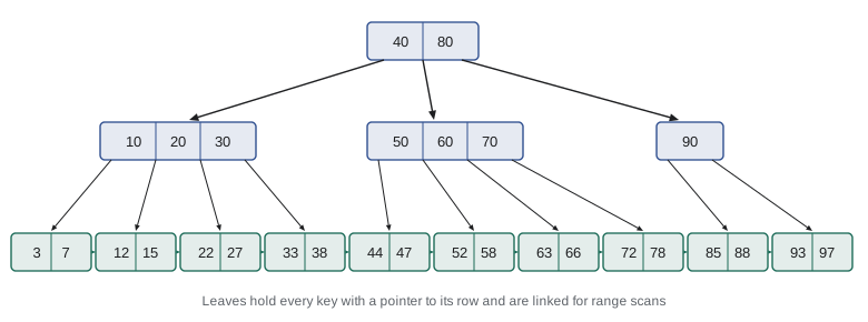
import math

def btree_height(n_keys, fanout):
    return max(1, math.ceil(math.log(n_keys, fanout)))

page_bytes, entry_bytes = 8192, 16            # key plus child pointer
fanout = page_bytes // entry_bytes             # entries per node
for n in (10_000, 1_000_000, 100_000_000, 10_000_000_000):
    h = btree_height(n, fanout)
print(f"{n:>14,} keys: height {h} -> about {h} page reads per lookup (fan-out {fanout})") 10,000 keys: height 2 -> about 2 page reads per lookup (fan-out 512)
1,000,000 keys: height 3 -> about 3 page reads per lookup (fan-out 512)
100,000,000 keys: height 3 -> about 3 page reads per lookup (fan-out 512)
10,000,000,000 keys: height 4 -> about 4 page reads per lookup (fan-out 512)Searching a B+-tree for a key reads one node per level, so a lookup among ten billion keys costs about four page reads, and the top levels are almost always in the buffer pool. Inserts and deletes keep the tree balanced by splitting full nodes and merging under-full ones, in time proportional to the height. A range query, such as grades between 80 and 89, descends once to the first matching leaf and then reads leaves sequentially. A B+-tree index helps equality conditions, range conditions, ORDER BY on the indexed columns and MIN or MAX queries.
Indexes in practice
Indexes are created with CREATE INDEX name ON table(columns), and most systems automatically index primary keys and UNIQUE columns, because enforcing uniqueness needs a fast lookup. An index on several columns is sorted by the first column, then the second within it, and so on, like a phone book sorted by last name then first name. It can therefore be used for conditions on a leftmost prefix of its columns: an index on (dept_id, credits) helps WHERE dept_id = 'CS' and WHERE dept_id = 'CS' AND credits > 50, but not WHERE credits > 50 alone. An index that contains every column a query needs is covering, and the DBMS can answer the query from the index without touching the table.
import random, sqlite3

random.seed(291)
con = sqlite3.connect(":memory:")
con.execute("CREATE TABLE enrollment (student_id INTEGER, sec_id INTEGER, grade INTEGER)")
con.executemany("INSERT INTO enrollment VALUES (?, ?, ?)",
                [(random.randint(1, 20000), random.randint(1, 900), random.randint(40, 100))
                 for _ in range(100_000)])

def plan(sql):
    return " | ".join(row[3] for row in con.execute("EXPLAIN QUERY PLAN " + sql))

q1 = "SELECT grade FROM enrollment WHERE student_id = 4242"
q2 = "SELECT student_id FROM enrollment WHERE sec_id = 17 AND grade >= 90"
q3 = "SELECT student_id FROM enrollment WHERE grade >= 90"
print("before:", plan(q1))
con.execute("CREATE INDEX enr_student ON enrollment(student_id)")
con.execute("CREATE INDEX enr_sec_grade ON enrollment(sec_id, grade, student_id)")
print("after :", plan(q1))
print("q2    :", plan(q2))
print("q3 :", plan(q3))before: SCAN enrollment after : SEARCH enrollment USING INDEX enr_student (student_id=?) q2 : SEARCH enrollment USING COVERING INDEX enr_sec_grade (sec_id=? AND grade>?) q3 : SCAN enrollment
Before the index, SQLite must scan the whole table. Afterwards it searches the index for student_id = 4242. The second query uses the composite index on (sec_id, grade, student_id) for both conditions, and because the index also contains student_id, it is a covering index and the table is never touched. The third query's condition is on grade alone, which is not a leftmost prefix of the composite index, so SQLite cannot search it and falls back to a full scan of the table. An index on grade, or a composite index that starts with grade, would be needed for that query, if it is frequent enough to justify the cost.
Indexes are not free. Each one takes space, and every INSERT, UPDATE or DELETE must update every index on the table, so a table with ten indexes accepts writes far more slowly than one with two. Indexes on columns with few distinct values, such as a yes-or-no flag, rarely help, because a condition on them matches a large fraction of the rows and a scan is cheaper than following thousands of index pointers. The usual practice is to index primary and foreign keys (foreign keys are used in joins and in checking deletes), then add indexes for the conditions and sort orders of frequent, slow queries, verified by looking at their plans.
| Index type | Supports | Notes |
|---|---|---|
| B+-tree | Equality, ranges, ORDER BY, prefix LIKE 'abc%' | The default almost everywhere |
| Hash | Equality only | Used internally for hash joins; PostgreSQL offers hash indexes |
| Composite (multi-column) B+-tree | Conditions on a leftmost prefix of the columns | Column order matters |
| Covering index | Queries answerable from index columns alone | Avoids table lookups |
| Partial index | Rows matching a WHERE condition only | For example only active loans |
| Full-text, spatial, GIN/GiST | Text search, geometry, JSON and arrays | System-specific |
Worked problem
Choosing an index
The library's most frequent query is: SELECT * FROM loan WHERE card_no = ? AND returned IS NULL ORDER BY due_date. The loan table has 2 million rows; a member has at most a few dozen loans. Which index would you create?
Show solution
- The equality condition is on card_no, which is highly selective (a few dozen rows out of 2 million). It should be the first column.
- The ORDER BY is on due_date within one member; putting due_date second lets the index return rows already sorted.
- Rows with a non-NULL returned value are most of the table; a partial index restricted to unreturned loans keeps the index small (supported by SQLite and PostgreSQL).
CREATE INDEX loan_open_by_member ON loan(card_no, due_date) WHERE returned IS NULL;- Check the plan with EXPLAIN QUERY PLAN to confirm the index is used.
Answer: An index on (card_no, due_date), ideally partial on returned IS NULL, serves both the condition and the sort.
How joins are executed
Joins are the most expensive common operation, and a DBMS has several algorithms for them. A nested-loop join takes each row of the outer table and scans the inner table for matches: simple, and good when the outer side is small and the inner side has an index on the join column (an index nested-loop join). A hash join builds a hash table on the join column of the smaller input and then probes it with each row of the larger: fast for large equijoins with no useful index. A sort-merge join sorts both inputs on the join column and merges them in one pass, which is efficient when inputs are already sorted, for example by an index, and also works for range conditions. SQLite relies mainly on nested loops with automatic indexes; PostgreSQL, MySQL 8.0.18 and later, and other servers use all three.
import random
random.seed(7)
students = [(i, f"s{i}") for i in range(2000)]                      # (student_id, name)
enroll   = [(random.randrange(2000), random.randrange(500)) for _ in range(8000)]  # (student_id, sec_id)

# Nested loop: compare every pair
comparisons = 0; nl = 0
for s_id, _ in students:
    for e_sid, _ in enroll:
        comparisons += 1
        nl += (s_id == e_sid)
print(f"nested loop: {comparisons:,} comparisons, {nl} matches")

# Hash join: build on the smaller input, probe with the larger
table = {}
for s_id, name in students:
    table.setdefault(s_id, []).append(name)
probes = 0; hj = 0
for e_sid, _ in enroll:
    probes += 1
    hj += len(table.get(e_sid, []))
print(f"hash join : {len(students):,} inserts + {probes:,} probes, {hj} matches")nested loop: 16,000,000 comparisons, 8000 matches hash join : 2,000 inserts + 8,000 probes, 8000 matches
Query optimization
Between the SQL text and the result, the query processor parses the query, checks it against the catalogue, translates it into a relational algebra tree, rewrites that tree using equivalences such as those in lesson 2, and then chooses physical algorithms and a join order. For each candidate plan the optimizer estimates a cost, mostly the number of page reads, using statistics stored in the catalogue: the number of rows in each table, the number of distinct values in columns, and histograms of value distributions. The fraction of rows a condition is expected to keep is its selectivity; a highly selective condition (few rows) favours an index, a non-selective one favours a scan.
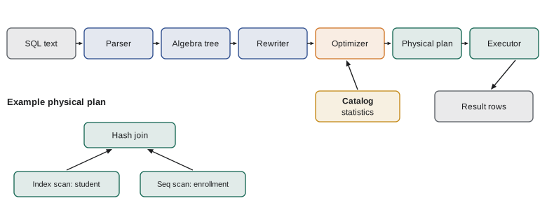
The number of possible join orders grows factorially with the number of tables, so optimizers search cleverly, classically with dynamic programming over subsets of tables as in IBM's System R, and with heuristics for very large queries. Estimates can be wrong, especially when statistics are stale or columns are correlated, and a wrong estimate can pick a bad plan. That is why systems provide ANALYZE (in SQLite, PostgreSQL and MySQL) to refresh statistics, and EXPLAIN (or EXPLAIN QUERY PLAN in SQLite) to show the chosen plan. Reading the plan, not guessing, is the first step in fixing a slow query.
Worked problem
Estimating selectivity
enrollment has 1,000,000 rows. The catalogue records 20,000 distinct student_id values and grades spread roughly evenly from 40 to 100. Estimate the rows returned by (a) WHERE student_id = 4242 and (b) WHERE grade >= 90, and say which is a better candidate for an index lookup.
Show solution
- (a) Assuming a uniform distribution, an equality on a column with 20,000 distinct values keeps about 1/20,000 of the rows: 1,000,000 / 20,000 = 50 rows.
- (b) Grades 90 to 100 cover 11 of the 61 possible values, about 18 per cent: roughly 180,000 rows.
- Fetching 50 rows through an index costs a few index pages plus up to 50 table pages. Fetching 180,000 rows through an index could cost up to 180,000 random page reads, more than scanning the whole table sequentially.
Answer: About 50 rows for (a), a good index candidate; about 180,000 rows for (b), where a full scan is likely cheaper. Optimizers make exactly this comparison using catalogue statistics.
Common mistakes
MistakeAdding an index to every column "just in case".
InsteadEach index slows every write and uses space. Index keys, foreign keys and the conditions of frequent slow queries, and verify with plans.
MistakeExpecting a composite index on (a, b) to help a condition on b alone.
InsteadA composite B+-tree is sorted by a first; only conditions on a leftmost prefix can use it for searching.
MistakeIndexing a low-selectivity column such as a boolean flag.
InsteadA condition matching a large fraction of rows is cheaper to answer with a scan; consider a partial index instead.
MistakeGuessing why a query is slow.
InsteadRun EXPLAIN (EXPLAIN QUERY PLAN in SQLite) and read the actual plan; refresh statistics with ANALYZE if estimates look wrong.
MistakeForgetting to index foreign keys used in joins.
InsteadJoins and referential checks on delete use the foreign key column; without an index each check can scan the child table.
Summary and key terms
- Storage devices are orders of magnitude slower than memory, so query cost is dominated by page reads; data is stored and cached in fixed-size pages.
- The buffer pool keeps hot pages in memory; heap files require full scans to find rows without an index.
- B+-trees are balanced, shallow trees with linked leaves, supporting equality and range searches in a handful of page reads.
- Composite indexes serve leftmost prefixes; covering indexes answer queries without table access; partial indexes cover selected rows.
- Indexes speed reads but slow writes and use space; index keys, foreign keys and frequent query conditions, verified with plans.
- Joins use nested-loop (with or without an index), hash or sort-merge algorithms, chosen by input sizes and available indexes.
- The optimizer rewrites queries and chooses plans using catalogue statistics and selectivity estimates; EXPLAIN shows the plan and ANALYZE refreshes statistics.
- Page
- The fixed-size unit in which a DBMS reads and writes data, typically 4 to 16 KB.
- Buffer pool
- Memory in which the DBMS caches pages read from storage.
- Heap file
- A table file with records stored in no particular order.
- Full table scan
- Reading every page of a table to answer a query.
- B+-tree
- A balanced tree index with keys in interior nodes and linked leaves holding entries.
- Fan-out
- The number of children per node in a tree index.
- Covering index
- An index containing every column a query needs.
- Selectivity
- The fraction of rows a condition is expected to keep.
- Hash join
- A join that builds a hash table on one input and probes it with the other.
- Query plan
- The tree of physical operators the DBMS uses to execute a query.
Practice problems
Work each problem on paper first, then reveal the answer to check.
A table has 2,000,000 rows of 250 bytes on 8 KB pages. About how many pages does it occupy?
Show answer
8192 // 250 = 32 rows per page, so about 62,500 pages.
With fan-out 400, what is the height of a B+-tree over 50 million keys?
Show answer
log base 400 of 50,000,000 is about 2.96, so height 3.
Which of these can use an index on (last_name, first_name): WHERE first_name = 'Ava', or WHERE last_name = 'Okafor'?
Show answer
Only the condition on last_name, the leftmost column.
Why do indexes slow down inserts?
Show answer
Every insert must also add an entry to every index on the table.
What does a covering index avoid?
Show answer
Looking up the table rows, because all needed columns are in the index.
When is a hash join preferable to an index nested-loop join?
Show answer
For large equijoins where no useful index exists on the inner table's join column.
Why might an optimizer ignore an index on a condition that matches 40% of rows?
Show answer
Following that many index pointers costs more random reads than one sequential scan.
What command shows SQLite's chosen plan for a query?
Show answer
EXPLAIN QUERY PLAN followed by the query.
Why should foreign key columns usually be indexed?
Show answer
They are used in joins and in checking deletes of the referenced rows.
What is the purpose of ANALYZE?
Show answer
To refresh the statistics the optimizer uses for cost estimates.
Lesson quiz · 5 questions
Score 60% or more to complete this lesson.
Create a free account to save your progress, take quizzes and earn a certificate.