
CMP-240 · Lesson 11 of 12 · 22 min
Sinusoids, phasors and impedance
Transient analysis tells you how a circuit responds to a single step. Many questions are instead about steady repeating signals: how much of the buck regulator's 400 kHz ripple reaches the radar's supply pin, how well a capacitor filters noise at 100 MHz, what fraction of a sensor signal survives a filter. Sinusoids are the key to all of these, for two reasons. A linear circuit driven by a sinusoid responds, once transients die away, with a sinusoid of the same frequency, changed only in amplitude and phase. And any repeating waveform, including a square clock signal, can be built from a sum of sinusoids, so by superposition the response to one sinusoid tells you the response to everything. Phasors and impedance turn the calculus of AC circuits into the algebra of complex numbers.
Describing a sinusoid
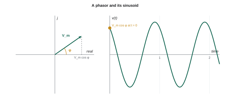
A sinusoidal voltage is described by its amplitude V_m, its angular frequency ω in radians per second, and its phase φ in radians or degrees. The ordinary frequency f in hertz is ω/2π, and the period T is 1/f. The phase says where the waveform is in its cycle at t = 0, and the difference in phase between two sinusoids of the same frequency says which one leads, reaching its peaks earlier.
The root-mean-square (RMS) value of a waveform is the steady DC value that would deliver the same average power to a resistor. For a sinusoid it is the amplitude divided by √2. Mains voltages are always quoted as RMS: North American 120 V outlets have a peak of about 170 V. Multimeters read RMS too, but only true-RMS meters read it correctly for non-sinusoidal waveforms such as the regulator's triangular ripple.
Phasors
Euler's formula, e^(jθ) = cos θ + j sin θ, links sinusoids to complex numbers. Engineers write the imaginary unit as j, because i is taken by current. A sinusoid V_m cos(ωt + φ) is the real part of V_m e^(jφ) e^(jωt). In a linear circuit every voltage and current shares the same e^(jωt) factor, so it can be dropped, leaving the complex number V = V_m∠φ, the phasor. The phasor carries amplitude and phase; the frequency is understood from the context.
The great simplification is that differentiation becomes multiplication by jω. Differentiating e^(jωt) gives jω e^(jωt), so the derivative of any sinusoid corresponds to its phasor multiplied by jω, and integration corresponds to division by jω. A differential equation in time becomes an algebraic equation in phasors. Phasors add like vectors, and multiplication multiplies the magnitudes and adds the angles, which is easiest in polar form; addition is easiest in rectangular form. Converting between the two forms is the main arithmetic of AC analysis.
Impedance
With phasors, each element's voltage-current relationship becomes Ohm's law with a complex resistance called impedance, Z = V/I, measured in ohms. A resistor's impedance is just R. For a capacitor, i = C dv/dt becomes I = jωC V, so Z = 1/(jωC): the capacitor's impedance falls as frequency rises, and its current leads its voltage by 90°. For an inductor, v = L di/dt becomes V = jωL I, so Z = jωL: the impedance rises with frequency, and the current lags the voltage by 90°. The imaginary part of an impedance is called reactance, X.
Impedance captures the limiting behaviours from lesson 8 in one formula. At DC (ω = 0) a capacitor's impedance is infinite, an open circuit, and an inductor's is zero, a short circuit. At very high frequencies the capacitor approaches a short and the inductor an open. This is exactly why a decoupling capacitor shorts fast noise to ground while leaving the DC supply untouched, and why an inductor in a supply line blocks noise while passing DC.
| Element | Impedance | At DC | At high frequency | Current relative to voltage |
|---|---|---|---|---|
| Resistor | R | R | R | In phase |
| Capacitor | 1/(jωC) | Open circuit | Short circuit | Leads by 90° |
| Inductor | jωL | Short circuit | Open circuit | Lags by 90° |
AC circuit analysis
Because impedances obey Ohm's law and phasors obey Kirchhoff's laws, every technique from lessons 2 to 6 works unchanged with complex numbers. Impedances combine in series and parallel like resistances, dividers divide, nodal and mesh analysis apply, superposition holds and Thévenin equivalents exist. The procedure is: convert sources to phasors, convert elements to impedances at the source frequency, solve the circuit with complex arithmetic, and convert the result back to a sinusoid if needed. Admittance, Y = 1/Z, measured in siemens, plays the role of conductance and is convenient for parallel combinations and for nodal analysis.
Worked problem
An RC voltage divider at one frequency
A 1 kΩ resistor in series with a 100 nF capacitor is driven by a 2 V amplitude, 1 kHz sinusoid, and the output is taken across the capacitor. Find the output amplitude and phase.
Show solution
- \[\omega = 2\pi(1000) = 6283\ \text{rad/s}, \qquad Z_C = \frac{1}{j(6283)(100 \times 10^{-9})} = -j1592\ \Omega\]
- \[\mathbf{V}_o = 2\angle 0^\circ \times \frac{-j1592}{1000 - j1592}\]
- \[1000 - j1592 = 1880\angle{-57.9^\circ}, \qquad -j1592 = 1592\angle{-90^\circ}\]
- \[\mathbf{V}_o = 2 \times \frac{1592}{1880}\angle(-90^\circ + 57.9^\circ) = 1.69\angle{-32.1^\circ}\ \text{V}\]
Answer: The output is a 1.69 V amplitude sinusoid lagging the input by 32°. At this frequency the capacitor's reactance, 1592 Ω, is larger than the resistance, so most of the voltage still appears across it. At higher frequencies its reactance shrinks and so does the output, which is the low-pass behaviour of lesson 12.
Real capacitors at high frequency
Lesson 8 mentioned that a real capacitor has equivalent series resistance (ESR) and equivalent series inductance (ESL). With impedance these become easy to analyse: the capacitor is a series RLC circuit with impedance ESR + jωL_ESL + 1/(jωC). At low frequencies the capacitive term dominates and the impedance falls as frequency rises; at the self-resonant frequency, 1/(2π√(L_ESL C)), the inductive and capacitive reactances cancel and the impedance equals the ESR; above it the inductance dominates and the impedance rises again. Above its self-resonance a capacitor behaves like an inductor, which is why small capacitors with low ESL are needed for the highest frequencies and why mounting inductance matters so much.
Worked problem
Where does the 100 nF decoupling capacitor stop working?
A 100 nF 0603 ceramic capacitor has an ESR of 30 mΩ and, including its pads and vias, about 1.2 nH of ESL. Find its self-resonant frequency and its impedance at 1 MHz, at resonance and at 200 MHz.
Show solution
- \[f_{SR} = \frac{1}{2\pi\sqrt{1.2 \times 10^{-9} \times 100 \times 10^{-9}}} = \frac{1}{2\pi(1.095 \times 10^{-8})} = 14.5\ \text{MHz}\]
- At 1 MHz: X_C = 1/(2π × 10⁶ × 10⁻⁷) = 1.59 Ω and X_L = 2π × 10⁶ × 1.2 × 10⁻⁹ = 0.0075 Ω, so |Z| ≈ 1.58 Ω.
- At 14.5 MHz the reactances cancel: |Z| = ESR = 0.03 Ω.
- At 200 MHz: X_L = 1.51 Ω and X_C = 0.008 Ω, so |Z| ≈ 1.50 Ω, inductive.
Answer: The capacitor is most effective around 14.5 MHz, where its impedance falls to 30 mΩ. At 200 MHz, where the microcontroller's fastest current spikes have much of their energy, it looks like a 1.2 nH inductor with 1.5 Ω of impedance. That is why boards add a few smaller capacitors, 1 nF to 10 nF, which resonate higher, and why the chip package and a solid ground plane, with their own built-in capacitance, matter most at the highest frequencies.
# Complex impedances with Python's built-in complex numbers (j is written 1j)
import math, cmath

def Zc(C, f):  return 1 / (1j * 2 * math.pi * f * C)
def Zl(L, f):  return 1j * 2 * math.pi * f * L
def polar(z):  return "%.4g ohm at %+.1f deg" % (abs(z), math.degrees(cmath.phase(z)))

# 1. RC divider at 1 kHz
Vin = 2.0
Zr, Zcap = 1000.0, Zc(100e-9, 1e3)
Vo = Vin * Zcap / (Zr + Zcap)
print("RC divider output: %.3f V at %.1f deg" % (abs(Vo), math.degrees(cmath.phase(Vo))))

# 2. A real 100 nF ceramic capacitor: ESR + ESL + C
def Zcap_real(f, C=100e-9, esr=0.030, esl=1.2e-9):
    return esr + Zl(esl, f) + Zc(C, f)

f_sr = 1 / (2 * math.pi * math.sqrt(1.2e-9 * 100e-9))
print("self-resonance %.1f MHz" % (f_sr / 1e6))
for f in (1e5, 1e6, 1e7, f_sr, 5e7, 2e8):
    print("  %9.0f kHz: |Z| = %s" % (f / 1e3, polar(Zcap_real(f))))

# 3. Adding a 1 nF capacitor in parallel extends the low-impedance range
def par(a, b): return a * b / (a + b)
for f in (5e7, 1e8, 2e8):
    z = par(Zcap_real(f), Zcap_real(f, C=1e-9, esr=0.08, esl=0.6e-9))
print(" 100 nF || 1 nF at %3.0f MHz: |Z| = %.3f ohm" % (f / 1e6, abs(z)))RC divider output: 1.693 V at -32.1 deg
self-resonance 14.5 MHz
100 kHz: |Z| = 15.91 ohm at -89.9 deg
1000 kHz: |Z| = 1.584 ohm at -88.9 deg
10000 kHz: |Z| = 0.08897 ohm at -70.3 deg
14529 kHz: |Z| = 0.03 ohm at +0.0 deg
50000 kHz: |Z| = 0.3465 ohm at +85.0 deg
200000 kHz: |Z| = 1.5 ohm at +88.9 deg
100 nF || 1 nF at 50 MHz: |Z| = 0.391 ohm
100 nF || 1 nF at 100 MHz: |Z| = 1.839 ohm
100 nF || 1 nF at 200 MHz: |Z| = 0.093 ohmThe last lines of the output hold a surprise. Adding the 1 nF capacitor cuts the impedance at 200 MHz from 1.5 Ω to under 0.1 Ω, but near 100 MHz the combination is worse than either part alone, at about 1.8 Ω. Between the two self-resonant frequencies the large capacitor already behaves like an inductor while the small one is still a capacitor, and the pair forms a parallel resonance, called an anti-resonance. Power-integrity engineers plot the impedance of the whole decoupling network against frequency to find and damp peaks like this one.
Why sinusoids describe digital signals
A square wave is not a sinusoid, but Fourier analysis, covered properly in ELE-250 and CMP-272, shows that a square wave of frequency f is the sum of sinusoids at f, 3f, 5f and so on, with amplitudes falling as 1/n. The faster the edges, the more high harmonics matter: a useful estimate says that a signal's significant frequency content extends to about 0.35/t_r, where t_r is the 10–90 percent rise time. The radar clock's 1 ns edges therefore contain energy up to about 350 MHz even though the clock itself runs at only 4 MHz. Analysing a circuit's impedance up to that frequency, one sinusoid at a time, tells you how it will treat the real digital signal.
The same idea explains a common surprise on the bench. A handheld multimeter set to AC volts reports an RMS value, but many inexpensive meters calculate it by measuring the average of the rectified waveform and multiplying by 1.11, the ratio that is correct only for a pure sinusoid. On a 3.3 V square wave with a 50 percent duty cycle, whose true AC RMS value is 1.65 V, such a meter reads about 1.83 V, roughly 11 percent high; on the narrow current pulses drawn by the NS-4's radio it can be wrong by a factor of two or more. A true-RMS meter, or an oscilloscope's RMS measurement, avoids the error. Phasor values are always the RMS or peak values of a pure sinusoid at one frequency, so when a measurement and a phasor calculation disagree, the first question is whether the waveform being measured really is sinusoidal.
Common mistakes
MistakeAdding phasors in polar form by adding magnitudes.
InsteadConvert to rectangular form to add; use polar form to multiply and divide.
MistakeUsing degrees and radians inconsistently.
InsteadKeep ωt in radians; convert phase angles explicitly when quoting degrees.
MistakeTreating a capacitor as an ideal capacitance at all frequencies.
InsteadInclude ESR and ESL; above self-resonance the part behaves like an inductor.
MistakeForgetting that phasor analysis applies only in steady state at one frequency.
InsteadFor transients use the time-domain methods; for several frequencies analyse each and superpose.
MistakeAssuming a slow clock has only low-frequency content.
InsteadThe spectrum depends on edge speed; content extends to about 0.35/t_r.
Summary and key terms
- A sinusoid is described by amplitude, frequency and phase; its RMS value is the amplitude divided by √2.
- A phasor V_m∠φ represents a sinusoid at a known frequency; differentiation becomes multiplication by jω.
- Impedances: Z_R = R, Z_C = 1/(jωC), Z_L = jωL; all circuit laws and methods work with complex impedances.
- Real capacitors have ESR and ESL and self-resonate; above resonance they behave inductively.
- Digital edges contain frequencies up to about 0.35/t_r, so impedance at high frequencies matters to digital design.
- Phasor
- A complex number giving the amplitude and phase of a sinusoid at a known frequency.
- Impedance
- The ratio of voltage phasor to current phasor, Z = R + jX.
- Reactance
- The imaginary part of impedance, positive for inductors and negative for capacitors.
- Admittance
- The reciprocal of impedance, Y = 1/Z.
- RMS value
- The DC value that delivers the same average power to a resistor.
- Self-resonant frequency
- The frequency at which a component's parasitic inductance and capacitance cancel.
- Knee frequency
- An estimate, 0.35/t_r, of the highest significant frequency in a digital edge.
Practice problems
Work each problem on paper first, then reveal the answer to check.
Write 5 cos(2π·50t − 30°) as a phasor and give its RMS value.
Show answer
5∠−30°; RMS 3.54.
Find the impedance of a 10 µH inductor at 400 kHz.
Show answer
j2π(4 × 10⁵)(10 × 10⁻⁶) ≈ j25.1 Ω.
Find the impedance of 10 Ω in series with 1 µF at 10 kHz, in polar form.
Show answer
10 − j15.9 = 18.8∠−57.8° Ω.
What is the self-resonant frequency of a 10 nF capacitor with 0.8 nH of ESL?
Show answer
1/(2π√(8 × 10⁻¹⁸)) ≈ 56 MHz.
Estimate the knee frequency for a 2.5 ns rise time.
Show answer
0.35/2.5 ns = 140 MHz.
Lesson quiz · 5 questions
Score 60% or more to complete this lesson.
Create a free account to save your progress, take quizzes and earn a certificate.