Rivers, lakes and the dissolved oxygen sag

When a city or factory discharges organic waste into a river, bacteria in the river begin to break it down, and they use dissolved oxygen to do it. At the same time, oxygen from the air dissolves back into the water through the surface. Just below the outfall, the bacteria consume oxygen faster than the air can replace it, so the dissolved oxygen falls. Farther downstream, as the waste is used up, reaeration catches up and the oxygen recovers. The resulting dip in the oxygen profile, called the dissolved oxygen sag, can kill fish if it falls too low. Predicting the sag was one of the first problems in environmental engineering, and the model developed by H. W. Streeter and Earle Phelps for the Ohio River in 1925 is still taught and used for screening today. This lesson develops that model and then turns to lakes, where stratification and nutrients, rather than flowing water, control water quality.

Martin has asked Nadia to check how the upgraded Brandon wastewater plant will affect oxygen in the Assiniboine River during a hot, dry August, the critical condition for fish. She also needs to show what would happen if the plant had to bypass partially treated wastewater during a breakdown.

Oxygen sources and sinks in a river

Several processes add oxygen to a river: reaeration from the atmosphere, photosynthesis by algae and aquatic plants during daylight, and inflow of oxygen-rich tributaries. Others remove it: decay of carbonaceous organic matter (carbonaceous BOD), nitrification of ammonia (nitrogenous BOD), respiration by algae and plants at night, and sediment oxygen demand from decaying material on the riverbed. The Streeter-Phelps model keeps only the two biggest processes for a polluted river, carbonaceous deoxygenation and atmospheric reaeration, which makes it simple enough to solve by hand while capturing the essential behaviour.

The oxygen deficit

It is convenient to work with the deficit, the difference between the saturation concentration and the actual dissolved oxygen:

Reaeration happens at a rate proportional to the deficit, k_a D, where k_a is the reaeration rate constant: the further the water is below saturation, the faster oxygen dissolves. Deoxygenation happens at the rate at which BOD is exerted, k_d L, where L is the ultimate BOD remaining and k_d is the deoxygenation rate constant, often taken equal to the laboratory BOD rate constant corrected for temperature. Treating the river as a plug flow reactor, so that time of travel t stands for distance downstream (x = ut), the deficit changes as:

The Streeter-Phelps equation

Solving this differential equation with an initial deficit D₀ and initial ultimate BOD L₀ just below the outfall gives the oxygen sag curve:

The lowest dissolved oxygen, the critical point, occurs when dD/dt = 0. Setting the derivative to zero gives the critical time:

Substituting t_c into the deficit equation gives the critical deficit D_c, and the minimum dissolved oxygen is DO_sat − D_c. The critical distance downstream is x_c = u t_c. If the logarithm's argument is less than one, the critical point is at the outfall itself, meaning the oxygen only recovers from there. The equations assume k_a and k_d differ; if they are equal, a limiting form is used.

Rate constants

The deoxygenation rate constant k_d is usually estimated from BOD tests and corrected to river temperature with θ ≈ 1.047. In shallow, fast rivers, bacteria growing on the bed can make the in-stream rate faster than the laboratory value. The reaeration rate constant depends on how turbulent the river is. Several empirical formulas exist; one of the oldest, from O'Connor and Dobbins, relates it to mean velocity u in m/s and depth H in m:

Shallow, fast rivers reaerate quickly and recover within a few kilometres; deep, slow rivers reaerate slowly and may carry a long sag. Reaeration depends less on temperature than deoxygenation (θ ≈ 1.024 compared with 1.047), so warm weather tends to deepen the sag, while the saturation concentration also falls in warm water.

Mixing at the outfall

Before applying the equations, the river and effluent are mixed using the flow-weighted averages of lesson 3. The ultimate BOD, dissolved oxygen and temperature are each averaged, and the saturation concentration is found at the mixed temperature.

Nadia then runs the model for normal operation and for a bypass in which the effluent's ultimate BOD rises to 150 mg/L.

# Streeter-Phelps dissolved oxygen sag for two effluent scenarios
import math
TAB = [(0, 14.62), (5, 12.77), (10, 11.29), (15, 10.08), (20, 9.09), (25, 8.26), (30, 7.56)]
def do_sat(T):                       # mg/L at sea level, linear interpolation
    for (a, x), (b, y) in zip(TAB, TAB[1:]):
        if a <= T <= b:
            return x + (y - x) * (T - a) / (b - a)

Qr, Lr, DOr, Tr = 3.0, 2.0, 7.9, 22.0      # river: m3/s, mg/L, mg/L, C
Qe, DOe, Te = 0.42, 2.0, 24.0              # effluent
u, H = 0.25, 1.8                           # velocity m/s, depth m
for label, Le in (("normal", 50.0), ("bypass", 150.0)):
    Q = Qr + Qe
    L0 = (Qr * Lr + Qe * Le) / Q
    T = (Qr * Tr + Qe * Te) / Q
    Ds = do_sat(T)
    D0 = Ds - (Qr * DOr + Qe * DOe) / Q
    kd = 0.30 * 1.047 ** (T - 20)
    ka = 3.93 * u ** 0.5 / H ** 1.5 * 1.024 ** (T - 20)
    D = lambda t: kd * L0 / (ka - kd) * (math.exp(-kd * t) - math.exp(-ka * t)) + D0 * math.exp(-ka * t)
    tc = math.log(ka / kd * (1 - D0 * (ka - kd) / (kd * L0))) / (ka - kd)
    xc = u * 86.4 * tc                     # km
    print(f"{label}: L0 = {L0:.1f} mg/L, critical point {xc:.0f} km downstream, minimum DO = {Ds - D(tc):.1f} mg/L")
    print("   km:  " + "  ".join(f"{x:4d}" for x in (0, 10, 20, 40, 60, 100)))
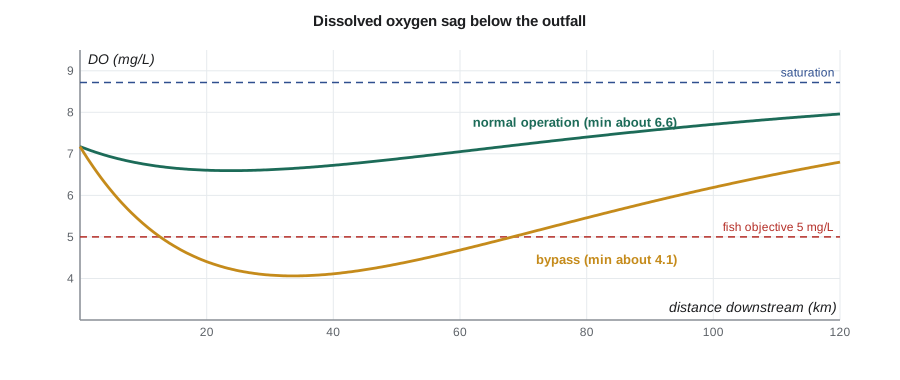
    print("   DO:  " + "  ".join(f"{Ds - D(x / (u * 86.4)):4.1f}" for x in (0, 10, 20, 40, 60, 100)))

normal: L0 = 7.9 mg/L, critical point 24 km downstream, minimum DO = 6.6 mg/L
   km:     0    10    20    40    60   100
   DO:   7.2   6.8   6.6   6.7   7.1   7.7
bypass: L0 = 20.2 mg/L, critical point 34 km downstream, minimum DO = 4.1 mg/L
   km:     0    10    20    40    60   100
   DO:   7.2   5.3   4.4   4.1   4.7   6.2

Under normal operation the oxygen falls to about 6.6 mg/L roughly 24 km downstream, comfortably above a typical objective of 5 to 6 mg/L for warm-water fish, and recovers within about 100 km. During a bypass, the ultimate BOD below the outfall rises to about 20 mg/L and the minimum falls to about 4.1 mg/L near 34 km, below the objective. Nadia's report recommends standby equipment and storage so that the plant never needs to bypass in late summer, and suggests checking the model against a field survey of oxygen along the river.

Limits of the model

The Streeter-Phelps model is a screening tool. It ignores nitrogenous BOD, which can be as large as the carbonaceous demand in effluents that are not nitrified; algal photosynthesis and respiration, which produce large daily swings in oxygen in nutrient-rich rivers, with supersaturation in the afternoon and the lowest values just before dawn; sediment oxygen demand; tributaries and other outfalls; and ice cover, which almost stops reaeration on prairie rivers in winter and can make late winter, not summer, the critical season. Modern studies use computer models such as QUAL2K, or the EPA's WASP, which include these processes and are calibrated against field surveys, but the structure is the same: mass balances on BOD, ammonia and oxygen in a series of reaches.

Lakes and reservoirs

Lakes behave very differently from rivers because water stays in them for months or years. In summer, many lakes in Canada and the northern United States stratify: the sun warms the surface layer, the epilimnion, which floats on the colder, denser bottom layer, the hypolimnion, separated by a zone of rapid temperature change, the thermocline. The layers barely mix, so the hypolimnion is cut off from the atmosphere for the whole summer. Organic matter settling from the surface decays there and can strip the bottom water of oxygen. In autumn the surface cools, the layers reach the same density and wind mixes the whole lake, a process called turnover; a similar turnover often follows ice-out in spring.

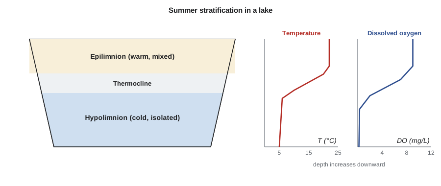
When the hypolimnion runs out of oxygen, sediments release phosphorus, iron, manganese and hydrogen sulphide, feeding more algae when the lake turns over and causing taste and odour problems for water utilities that draw from the bottom. This is one reason reservoir intakes often have several gates at different depths.

Trophic status and phosphorus budgets

Lakes are classified by their productivity. Oligotrophic lakes are clear and nutrient-poor, with deep oxygenated water; eutrophic lakes are green, nutrient-rich and prone to oxygen depletion and algal blooms; mesotrophic lakes fall in between. Total phosphorus is the usual indicator. Ranges commonly used in Canadian guidance are below 10 µg/L for oligotrophic, 10 to 20 µg/L for mesotrophic, 20 to 35 µg/L for meso-eutrophic, 35 to 100 µg/L for eutrophic and above 100 µg/L for hypereutrophic lakes.

A simple steady-state phosphorus budget treats the lake as a CMFR in which phosphorus is lost to the outflow and to settling, with a settling rate proportional to concentration. If W is the phosphorus load (g/yr), Q the outflow (m³/yr), A the surface area (m²) and v_s an apparent settling velocity (m/yr), the lake concentration is: