
CIV-280 · Lesson 4 of 12 · 27 min
Reaction kinetics and natural decay
A mass balance tells you what goes in and out; kinetics tells you how fast things change inside. Bacteria die in a river, organic matter is consumed by microbes, chlorine reacts with pipe walls, radon decays in a basement and pesticides break down in soil, each at its own rate. Engineers need those rates to size treatment tanks, to predict how far downstream an outfall affects a river, and to estimate how long a contaminated site will take to recover. This lesson covers rate laws and reaction order, the first-order model that describes most environmental decay, half-life, the effect of temperature on rates, and how to estimate a rate constant from laboratory or field data.
Reaction rates and order
The rate of a reaction is the change in concentration per unit time. For many reactions, the rate depends on concentration raised to some power, called the order of the reaction:
Here k is the rate constant and n is the order. The minus sign shows that the concentration is decreasing. The order is usually found by experiment, not from the balanced equation, because most environmental processes involve many steps.
| Order | Rate law | Integrated form | Units of k | Examples |
|---|---|---|---|---|
| Zero | \(dC/dt = -k\) | \(C = C_0 - kt\) | mg/(L·d) | Reactions limited by enzyme or catalyst capacity |
| First | \(dC/dt = -kC\) | \(C = C_0 e^{-kt}\) | 1/d | Radioactive decay, bacterial die-off, BOD exertion, many pesticides |
| Second | \(dC/dt = -kC^2\) | \(1/C = 1/C_0 + kt\) | L/(mg·d) | Some reactions between two dissolved species |
In a zero-order reaction the concentration falls by the same amount each day, regardless of how much is left, so it reaches zero in a finite time. In a first-order reaction it falls by the same fraction each day, so it approaches zero gradually and never quite reaches it. First-order behaviour is so common in environmental systems that it is the default assumption unless data show otherwise.
First-order decay and half-life
Integrating the first-order rate law from an initial concentration C₀ gives exponential decay:
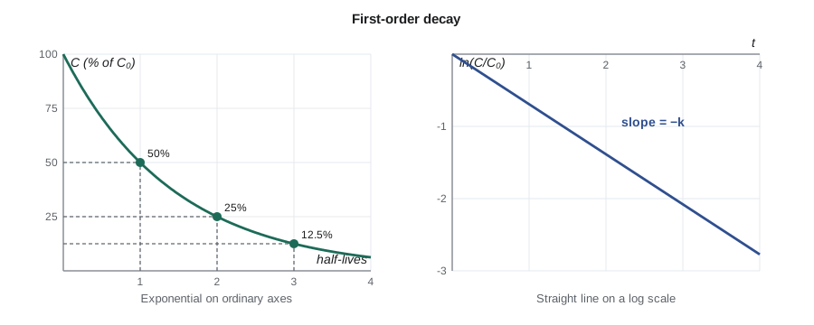
The half-life is the time for the concentration to fall to half its initial value. Setting C/C₀ = 1/2 gives a half-life that does not depend on the starting concentration:
After one half-life, 50 per cent remains; after two, 25 per cent; after three, 12.5 per cent; after ten, about 0.1 per cent. Engineers use the same arithmetic to describe how long a spill takes to fade, how quickly a disinfectant dissipates in a water main and how fast a radioactive isotope loses its activity.
Worked problem
Radon in a basement
Radon-222, a radioactive gas from uranium in soil and rock, decays with a half-life of 3.82 days. A sealed sample of basement air is taken to the laboratory, which measures it 10 days later. What fraction of the radon in the original sample is left when it is measured?
Show solution
- \[k = \frac{0.693}{3.82} = 0.181\ \text{d}^{-1}\]
- \[\frac{C}{C_0} = e^{-0.181 \times 10} = 0.163\]
Answer: Only about 16 per cent of the radon remains after ten days, so the laboratory must correct its measurement back to the sampling time. Radon is the leading cause of lung cancer in people who have never smoked, and both Health Canada and the EPA recommend testing homes and reducing levels above their action levels.
Bacterial die-off
Bacteria from sewage and animal manure gradually die in rivers and lakes because of sunlight, temperature, predation and lack of nutrients. Die-off is usually modelled as first order, with rate constants that vary widely, from about 0.5 per day in cold, turbid water to several per day in warm, clear water exposed to sunlight. Engineers use die-off rates to estimate how far downstream of a sewer overflow a beach or drinking water intake is at risk.
Worked problem
Distance for a 99 per cent reduction
E. coli from a combined sewer overflow die off in a river with a first-order rate constant of 1.2 per day. The river flows at 0.40 m/s. How long and how far must the water travel to reduce the bacteria by 99 per cent, assuming plug flow and no dilution?
Show solution
- \[e^{-kt} = 0.01 \quad\Rightarrow\quad t = \frac{\ln 100}{1.2} = 3.84\ \text{d} = 92\ \text{h}\]
- \[x = 0.40\ \text{m/s} \times 3.84 \times 86\,400\ \text{s} = 133\,000\ \text{m} \approx 133\ \text{km}\]
Answer: The water must travel almost four days and well over 100 km for die-off alone to remove 99 per cent of the bacteria. In reality dilution also lowers the concentration, but the result shows why overflows near intakes and beaches are taken so seriously.
Temperature and reaction rates
Most chemical and biological reactions speed up as temperature rises. The Arrhenius equation describes this in terms of an activation energy, but environmental engineers usually use a simpler empirical form, often called the van 't Hoff–Arrhenius relationship:
Here k₂₀ is the rate constant at 20 °C, T is the temperature in degrees Celsius, and θ is a temperature coefficient, typically between 1.02 and 1.09. A common value for biochemical oxygen demand is 1.047, which means the rate rises about 4.7 per cent for each degree of warming, roughly doubling every 15 °C. Temperature effects matter enormously in the prairies and northern states, where river temperatures swing from near freezing in winter to more than 20 °C in summer.
Worked problem
Slower decay in a cold river
A laboratory measures the BOD rate constant of a wastewater as 0.23 per day at 20 °C. Using θ = 1.047, estimate the rate constant in the river at 10 °C and at 25 °C.
Show solution
- \[k_{10} = 0.23 \times 1.047^{\,10-20} = 0.23 \times 0.632 = 0.145\ \text{d}^{-1}\]
- \[k_{25} = 0.23 \times 1.047^{\,25-20} = 0.23 \times 1.258 = 0.289\ \text{d}^{-1}\]
Answer: At 10 °C the organic matter is consumed about 37 per cent more slowly than at 20 °C, and at 25 °C about 26 per cent faster. Slower decay in cold water spreads oxygen demand over a longer reach of river, while warm water speeds decay but also holds less oxygen, which is why summer low flows are usually the critical condition.
Estimating a rate constant from data
Rate constants come from experiments. For a first-order reaction, taking the natural logarithm of C = C₀e^(−kt) gives ln C = ln C₀ − kt, a straight line in time. Plotting ln C against t, or C on a logarithmic axis, and fitting a line by least squares gives −k as the slope. If the points curve instead of falling on a line, the reaction is not first order, or more than one process is involved.
Joy ran a degradation test on the herbicide from lesson 3. She spiked lake water with the herbicide, kept it in the dark at the lake's summer temperature, and measured the concentration over two weeks.
| Day | 0 | 1 | 2 | 4 | 7 | 10 | 14 |
|---|---|---|---|---|---|---|---|
| Herbicide (µg/L) | 50.0 | 42.1 | 36.4 | 26.8 | 17.0 | 11.2 | 6.4 |
# Fit a first-order rate constant by least squares on ln(C) versus t
import math
t = [0, 1, 2, 4, 7, 10, 14]                    # days
C = [50.0, 42.1, 36.4, 26.8, 17.0, 11.2, 6.4]   # ug/L
y = [math.log(c) for c in C]
n = len(t)
tm, ym = sum(t) / n, sum(y) / n
slope = sum((a - tm) * (b - ym) for a, b in zip(t, y)) / sum((a - tm) ** 2 for a in t)
icept = ym - slope * tm
k = -slope
ss_res = sum((b - (icept + slope * a)) ** 2 for a, b in zip(t, y))
ss_tot = sum((b - ym) ** 2 for b in y)
print(f"k = {k:.3f} per day, fitted C0 = {math.exp(icept):.1f} ug/L")
print(f"half-life = {math.log(2) / k:.1f} days, R^2 = {1 - ss_res / ss_tot:.4f}")k = 0.147 per day, fitted C0 = 48.8 ug/L half-life = 4.7 days, R^2 = 0.9994
The fit gives k ≈ 0.147 per day and a half-life of about 4.7 days, with an R² above 0.999, so the first-order model describes the data very well. Joy's earlier estimate of 0.10 per day, used in lesson 3, was conservative; with the measured rate, the lake concentration would be lower. Field rates, however, often differ from laboratory rates because sunlight, sediments and changing temperature all play a part, so Nadia keeps both values and reports the range.
Kinetics in treatment and distribution
Kinetics also drives treatment design. In 1908 Harriette Chick showed that bacteria exposed to a disinfectant die off approximately as a first-order reaction in time, and Herbert Watson added the effect of disinfectant concentration. The resulting Chick-Watson model is usually written with the product of concentration and contact time:
Here N is the number of surviving organisms, C the disinfectant concentration and t the contact time. Because only the product C × t appears, a short contact at a high dose achieves the same kill as a long contact at a low dose. This is the basis of the CT concept used to design chlorine contact tanks in lesson 7. Disinfection is usually described in log reductions: a 2-log reduction removes 99 per cent of the organisms, a 3-log reduction 99.9 per cent and a 4-log reduction 99.99 per cent.
Chlorine itself decays in a water main as it reacts with organic matter in the water and with biofilm and corrosion products on the pipe walls. Utilities model this as first-order decay, with a bulk rate measured in bottles and a wall rate that depends on pipe material and age. If the chlorine residual at the far ends of the system falls too low, utilities add booster chlorination stations or flush the mains. Iron pipes that are old and heavily tuberculated can consume chlorine many times faster than new plastic pipe, which is one reason residual monitoring is part of every distribution system's routine.
Worked problem
Chlorine residual at the end of a long main
Water leaves a reservoir with a free chlorine residual of 1.2 mg/L. The combined bulk and wall decay rate in a long rural transmission main is 0.40 per day, and water takes 30 hours to reach the last farm on the line. What residual reaches the farm?
Show solution
- \[t = 30/24 = 1.25\ \text{d}\]
- \[C = 1.2\,e^{-0.40 \times 1.25} = 1.2 \times 0.607 = 0.73\ \text{mg/L}\]
Answer: About 0.7 mg/L of free chlorine reaches the farm, enough to protect the water in most jurisdictions, which typically expect a detectable residual of at least 0.2 mg/L throughout the system. In summer, warmer water would speed decay, and the residual should be checked again.
Kinetics in the real world
Environmental systems rarely behave as neatly as a single first-order reaction. Microbial growth follows saturation kinetics: at low substrate concentrations the rate is roughly first order, but at high concentrations the microbes are working as fast as they can and the rate levels off, approaching zero order. The Monod equation, used in wastewater design, captures this behaviour. Some pollutants degrade in steps, forming intermediates that may be more toxic than the parent compound; trichloroethylene, a common groundwater solvent, can break down to vinyl chloride, a known human carcinogen, before degrading further. Sorption to soil, volatilization to air and photolysis by sunlight may all act at once. Engineers handle this complexity by measuring rates under realistic conditions, using conservative values in design and checking predictions with monitoring.
Persistence is the flip side of decay. Substances with half-lives of years or decades in the environment, such as PCBs, mercury and many per- and polyfluoroalkyl substances (PFAS), accumulate in sediments and food chains. Some become more concentrated at each step up the food chain, a process called biomagnification, so that fish-eating birds and people who eat a lot of fish receive the highest doses. For these substances, preventing release is far more effective than any downstream treatment.
Common mistakes
MistakeUsing a zero-order equation for a first-order process.
InsteadFirst-order decay removes a constant fraction per unit time, not a constant amount.
MistakeApplying a rate constant measured at 20 °C directly to a cold river.
InsteadCorrect for temperature with k_T = k₂₀ θ^(T − 20).
MistakeUsing log₁₀ in the half-life formula.
InsteadThe half-life is ln 2/k with the natural logarithm; using log₁₀ requires a factor of 2.303.
MistakeFitting a straight line to C versus t for first-order data.
InsteadFit ln C against t; a straight line on that plot confirms first-order behaviour.
Summary and key terms
- Reaction order describes how rate depends on concentration; most environmental decay is approximately first order.
- First-order decay gives C = C₀e^(−kt) and a constant half-life t½ = 0.693/k.
- Bacterial die-off, radioactive decay and many pesticides follow first-order kinetics.
- Rate constants change with temperature: k_T = k₂₀θ^(T − 20), with θ ≈ 1.047 for BOD.
- Rate constants are estimated from the slope of ln C against time.
- Persistent substances with long half-lives accumulate in sediments and food chains.
- Rate constant
- The proportionality constant k in a rate law.
- Reaction order
- The power to which concentration is raised in a rate law.
- First-order reaction
- A reaction whose rate is proportional to the concentration of one reactant.
- Half-life
- The time required for a concentration to fall to half its initial value.
- Temperature coefficient
- The factor θ by which a rate constant changes per degree Celsius.
- Die-off
- The natural decline in numbers of bacteria or viruses in the environment.
- Persistence
- The tendency of a substance to remain in the environment without breaking down.
- Biomagnification
- The increase in concentration of a substance at each higher level of a food chain.
Practice problems
Work each problem on paper first, then reveal the answer to check.
A pesticide has a half-life of 30 days in soil. What is its first-order rate constant?
Show answer
\(0.693/30 = 0.0231\) per day.
What fraction of that pesticide remains after 90 days?
Show answer
Three half-lives: \(0.5^3 = 0.125\), or 12.5 per cent.
A rate constant is 0.30 per day at 20 °C. Estimate it at 5 °C with θ = 1.047.
Show answer
\(0.30 \times 1.047^{-15} = 0.30 \times 0.502 = 0.151\) per day.
How many half-lives reduce a concentration by 99.9 per cent?
Show answer
About 10, because \(0.5^{10} = 0.001\).
A zero-order reaction removes 2 mg/L per hour from an initial 15 mg/L. How long until the concentration reaches zero?
Show answer
\(15/2 = 7.5\) h.
Why are laboratory decay rates often different from field rates?
Show answer
Field conditions such as sunlight, temperature swings, sediments, mixing and the microbial community differ from controlled laboratory tests.
Lesson quiz · 5 questions
Score 60% or more to complete this lesson.
Create a free account to save your progress, take quizzes and earn a certificate.