
CHE-380 · Lesson 4 of 12 · 21 min
Dispersion models and emergency planning
Once a source model gives the release rate, the next question is where the material goes. A vapour released into the open air is carried by the wind and mixed by turbulence until its concentration falls below levels that matter. Dispersion models estimate the concentration at each point downwind. They are used to decide how far a flammable cloud could reach before it is too lean to burn, which buildings could see harmful concentrations, how far an emergency plan should extend, and where gas detectors should be placed. In this lesson Theo and Nadia use the classic Gaussian models to estimate how far vapour from the ethyl acetate dike pool of lesson 3 could travel.
What controls dispersion
Three things control how fast a release dilutes. Wind speed sets how quickly the material is carried away and how much air it is mixed into per second: concentration is roughly inversely proportional to wind speed. Atmospheric stability sets how strongly the air mixes vertically. On a sunny afternoon the ground heats the air, warm air rises and turbulence is strong; the atmosphere is unstable and dispersion is rapid. On a clear night with light wind the ground cools the air near it, the air becomes stably stratified and vertical mixing is suppressed; a cloud can then travel long distances with little dilution. Surface roughness, from flat fields to buildings and tanks, adds mechanical turbulence and speeds mixing.
The density of the released material also matters. Most releases of solvent vapour at Kingfisher Bioenergy are slightly heavier than air once they cool by evaporation, and in still conditions they spread along the ground and into low areas such as sumps and trenches. Heavy gases such as propane and chlorine slump and spread sideways before they dilute, and need dense-gas models. Light or buoyant releases rise. The Gaussian models in this lesson apply to neutrally buoyant releases after they have mixed with enough air, which makes them suitable for screening the dike pool scenario but not for the early stage of a large dense release.
Stability classes
Pasquill and Gifford grouped atmospheric conditions into six stability classes from A, very unstable, to F, moderately stable, based on wind speed, sunlight and cloud cover. Class D, neutral, applies to overcast skies and moderate to strong winds at any time of day. Class F applies to clear nights with light winds. Many regulatory and company studies use two standard weather cases: D with a wind of about 5 m/s, and F with about 1.5 m/s. The F case usually gives the longest distances and is often used as a worst case for planning.
| Class | Description | Typical conditions |
|---|---|---|
| A | Very unstable | Strong sun, light wind |
| B | Unstable | Moderate sun, light to moderate wind |
| C | Slightly unstable | Daytime, moderate wind |
| D | Neutral | Overcast or strong wind, day or night |
| E | Slightly stable | Night, partial cloud, light wind |
| F | Stable | Clear night, light wind |
The Gaussian plume
For a continuous release at a steady rate \(Q\) into a steady wind \(u\), the concentration downwind is modelled as a plume whose cross-section has a Gaussian profile in the horizontal and vertical directions. For a release at ground level, the concentration on the ground directly downwind of the source at distance \(x\) is
where \(\sigma_y\) and \(\sigma_z\) are the horizontal and vertical dispersion coefficients, which grow with distance and depend on the stability class. For an elevated release at height \(H\), the ground-level centreline concentration is multiplied by \(\exp(-H^2/2\sigma_z^2)\), which is why tall stacks reduce ground concentrations close to the source. The dispersion coefficients are given by curves or by fitted formulas. Briggs' formulas for open country are widely used; for class D, for example, \(\sigma_y = 0.08x(1 + 0.0001x)^{-1/2}\) and \(\sigma_z = 0.06x(1 + 0.0015x)^{-1/2}\), with \(x\) in metres.
# Gaussian plume for a continuous ground-level release (Pasquill-Gifford, Briggs rural sigmas)
import math
def sig(cls, x):
    if cls == 'D': return 0.08 * x / math.sqrt(1 + 0.0001 * x), 0.06 * x / math.sqrt(1 + 0.0015 * x)
    if cls == 'F': return 0.04 * x / math.sqrt(1 + 0.0001 * x), 0.016 * x / (1 + 0.0003 * x)
def conc(Q, u, x, cls):           # ground level, on the plume axis, release at ground
    sy, sz = sig(cls, x)
    return Q / (math.pi * sy * sz * u)
Q = 0.26                          # kg/s, evaporation from the dike pool of lesson 3
M = 88.1
to_ppm = lambda c: c / (M / 1000) * 0.02445 * 1e6   # kg/m3 -> ppm at 25 C
print(" x (m)   D, 5 m/s (ppm)   F, 1.5 m/s (ppm)")
for x in (25, 50, 100, 200, 400, 800):
    print(f"{x:5d} {to_ppm(conc(Q, 5.0, x, 'D')):14.0f} {to_ppm(conc(Q, 1.5, x, 'F')):16.0f}")
# Distance to a concentration endpoint (bisection)
def dist(target, u, cls):
    lo, hi = 1.0, 20000.0
    for _ in range(60):
        mid = (lo + hi) / 2
        if to_ppm(conc(Q, u, mid, cls)) > target: lo = mid
        else: hi = mid
    return mid
lfl = 20_000.0    # ethyl acetate lower flammable limit 2.0 % by volume
for name, tgt in (("half the LFL (10,000 ppm)", lfl / 2), ("400 ppm, the 8-hour limit", 400.0)):
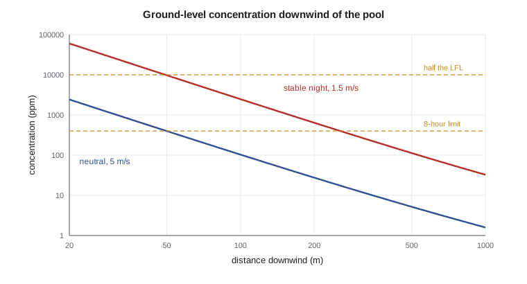
print(f"distance to {name}: D {dist(tgt, 5.0, 'D'):.0f} m, F {dist(tgt, 1.5, 'F'):.0f} m")x (m) D, 5 m/s (ppm) F, 1.5 m/s (ppm) 25 1562 38616 50 398 9738 100 103 2477 200 28 640 400 8 171 800 2 48 distance to half the LFL (10,000 ppm): D 10 m, F 49 m distance to 400 ppm, the 8-hour limit: D 50 m, F 255 m
With the pool evaporating 0.26 kg/s, the concentration 25 m downwind is about 1,600 ppm in class D with a 5 m/s wind, but about 39,000 ppm in class F with a 1.5 m/s wind: almost 25 times higher. Half the lower flammable limit, 10,000 ppm, is a common screening endpoint for flammable clouds, because the model gives time-averaged centreline values and real clouds have pockets richer than the average. It reaches about 10 m in class D and about 49 m in class F. The 8-hour exposure limit of 400 ppm reaches about 50 m and 255 m. These are rough estimates, but they already tell the team something important: on a calm night a flammable cloud from a dike fire could extend beyond the dike, toward the drum filling station 40 m away.
Worked problem
Plume concentration
A ground-level source releases 0.5 kg/s. At 200 m in class D with \(u = 4\) m/s, \(\sigma_y = 15.7\) m and \(\sigma_z = 10.2\) m. Find the centreline concentration in kg/m³.
Show solution
- \(C = 0.5/(\pi \times 15.7 \times 10.2 \times 4)\).
- \(C = 2.5 \times 10^{-4}\) kg/m³, or 0.25 g/m³.
Answer: About 0.25 g/m³; converting to ppm needs the molar mass.
Puffs and instantaneous releases
A sudden release, such as a vessel rupture, forms a puff that drifts downwind and grows as it travels. Its centre concentration is
for a ground-level puff of mass \(m\), where the factor 2 accounts for reflection from the ground. Puff dispersion coefficients differ from plume coefficients because a puff samples only the turbulence at its own scale. Puff models are used for catastrophic failures and for the early stage of short releases. The concentration at a point rises and falls as the puff passes, and the dose received depends on the time-integrated concentration.
Endpoints for flammable and toxic releases
A dispersion model gives concentrations; an endpoint says which concentrations matter. For flammable releases the endpoint is the lower flammable limit, often with a factor such as one half to allow for concentration fluctuations; within that zone an ignition source could ignite the cloud. For toxic releases, emergency planning uses endpoints for exposures of about an hour. The American Industrial Hygiene Association publishes emergency response planning guidelines, ERPGs, at three levels, and acute exposure guideline levels, AEGLs, are published for several exposure times. Level 1 corresponds to mild discomfort, level 2 to effects that could impair escape, and level 3 to life-threatening effects. Emergency plans commonly draw zones where the level 2 value could be exceeded, so that people there can be warned to shelter or evacuate.
In Canada, facilities storing listed substances above threshold quantities must prepare environmental emergency plans under Canada's Environmental Emergency Regulations under the Canadian Environmental Protection Act. Where it applies, the analysis of a worst-case release and alternative scenarios is reported, and the community is informed of the hazard. At Kingfisher Bioenergy the main hazards are flammable, and the emergency plan's zones are based on flammable cloud distances and thermal radiation, with toxic endpoints considered for the small ammonia and sulphuric acid inventories used for pH control.
Limits of simple models
Gaussian models assume a steady wind, flat terrain, a neutrally buoyant release and a concentration that has been averaged over several minutes. Real releases may be dense, jet-like or affected by buildings and tanks that create wakes and channel flow. Short-term peak concentrations can be several times the average. Near the source, the release behaves as a jet or a slumping cloud rather than a plume. Commercial consequence models handle many of these effects, and computational fluid dynamics is used for complex sites. Nadia uses the Gaussian estimates to screen the scenarios and to check the order of magnitude of results from the company's consequence software, and she treats any result within a factor of two of a decision threshold as needing more careful work.
Gas detection and dispersion
Dispersion models also guide where gas detectors go. A detector placed where a cloud rarely reaches is of little use, and a detector placed too close to a source may alarm on harmless small leaks. Practice uses the expected release points, the prevailing wind directions and the dense or buoyant character of the vapour to choose locations, often at a low height for heavier-than-air vapours such as ethyl acetate and near the boundaries of occupied areas. Detectors for flammable gas are usually set to alarm at 10 to 25 % of the LFL and to trip equipment or start ventilation at a higher level. Their response time, typically tens of seconds, must be counted in the isolation time used in the source model.
Weather data for the site help too. The meteorological records for Sarnia show the frequency of each wind direction and stability class through the year. Combining them with the dispersion results gives the fraction of the time that a cloud would travel toward each neighbour, which is an input to the risk calculations of lesson 11. Nadia points out that stable night conditions are common in the cold months at Sarnia, so the F-class case is not a rare extreme but a regular part of the year.
Elevated releases behave differently. The vent stack of the column's scrubber, studied in CHE-314, discharges at about 15 m. Its plume must travel some distance before it reaches the ground, and the highest ground concentration occurs downwind, where \(\sigma_z\) has grown to about the stack height divided by \(\sqrt{2}\). For the small flows from the scrubber, the ground concentrations are tiny, but the same method is used for permits under the ECA.
Using the results
The dispersion study changes three things in the tank farm design. First, gas detectors are added at the dike wall on the side facing the drum filling station, set to alarm at a fraction of the lower flammable limit. Second, the electrical area classification of lesson 7 is checked against the cloud distances, and the drum filling station's equipment is confirmed to be suitable for a classified area. Third, the emergency plan adds a response for a dike spill at night in calm weather: start the foam system early to cover the pool, which cuts the evaporation rate, and keep vehicles away from the downwind side. The study does not need precise numbers to justify these actions, only a clear picture of which way the hazard points.
Common mistakes
MistakeUsing a single weather case for planning.
InsteadCheck at least neutral daytime and stable night cases; F is often worst.
MistakeTreating the time-averaged centreline concentration as the peak.
InsteadAllow for fluctuations, for example by using half the LFL.
MistakeApplying a Gaussian model to the early stage of a dense gas release.
InsteadUse a dense-gas model until the cloud is dilute.
MistakeForgetting the reflection factor for a ground-level puff.
InsteadInclude the factor of 2 for ground reflection.
Summary and key terms
- Concentration falls with wind speed and with atmospheric mixing, which depends on stability.
- Classes A to F describe stability; D and F are common planning cases.
- The ground-level plume formula is \(C = Q/(\pi\sigma_y\sigma_zu)\).
- Half the LFL from the dike pool reaches about 10 m in class D and 49 m in class F.
- ERPGs and AEGLs set endpoints for emergency planning of toxic releases.
- Plume
- A continuous release carried downwind.
- Puff
- An instantaneous release that drifts downwind as a cloud.
- Stability class
- A category describing the vertical mixing of the atmosphere.
- Dispersion coefficient
- A length describing the spread of a plume in one direction.
- ERPG
- An emergency response planning guideline concentration for about one hour of exposure.
- Dense gas
- A release heavier than air that slumps and spreads along the ground.
Practice problems
Work each problem on paper first, then reveal the answer to check.
Halve the wind speed in the plume formula, other things equal. What happens to the concentration?
Show answer
It doubles, though the dispersion coefficients may also change.
Which stability class usually gives the longest hazard distances?
Show answer
F, stable night conditions.
Why do tall stacks reduce ground concentrations near the source?
Show answer
The plume must spread down before reaching the ground: the \(\exp(-H^2/2\sigma_z^2)\) factor.
Why is half the LFL used as a flammable endpoint?
Show answer
To allow for concentration fluctuations above the time average.
Name one situation where a Gaussian plume is not appropriate.
Show answer
A dense gas release close to the source, or flow among buildings.
What two design changes followed from the dispersion study?
Show answer
Gas detectors at the dike wall and a check of area classification at the drum station.
Lesson quiz · 5 questions
Score 60% or more to complete this lesson.
Create a free account to save your progress, take quizzes and earn a certificate.