Model serving, latency and throughput

An online model is part of a product, and products have speed requirements. A search page must return results in a few hundred milliseconds, a payment must be approved in well under a second, and an ad auction may allow a model only ten milliseconds. Meeting these requirements at reasonable cost is a systems problem: it depends on the model's execution time, but also on queueing, batching, network hops, feature lookups and how many replicas are running. This lesson covers latency budgets and percentiles, the queueing behaviour that makes servers slow down sharply as they get busy, batching, autoscaling, caching, and the choice of hardware. Optimizations specific to large language models, such as KV caching and speculative decoding, are covered in AI-410, Lesson 8.

Latency budgets and percentiles

End-to-end latency is the time from a user's action to the response. A model is only one part of it, so teams set a latency budget for each component. For a fraud check with a 300 ms limit, the budget might allow 20 ms for the network, 30 ms for feature lookups from the online store, 50 ms for the model, and leave the rest for the payment system itself.

Latency must be described by percentiles, not averages. The median (p50) is the typical request; the 99th percentile (p99) is the time within which 99 % of requests finish. Users experience the tail: a page that calls ten services is slow if any one of them is slow, so a 1-in-100 slow response from each service makes roughly 1 in 10 pages slow. Service level objectives (SLOs) are therefore stated as percentiles, for example "p99 latency below 50 ms over each five-minute window".

Where the time goes

A request to a model service passes through several stages: network transfer, request parsing, feature retrieval (often several lookups), preprocessing, waiting in a queue for a free worker, model execution, postprocessing and the response. Profiling usually shows that model execution is not the only, or even the main, cost. Feature lookups that run one after another, JSON parsing of large payloads, or Python preprocessing can dominate. The first optimizations are often the cheapest: fetch features in parallel or in one batched call, keep connections open, avoid repeated conversions, and move heavy preprocessing out of the request path.

Queueing: why busy servers are slow

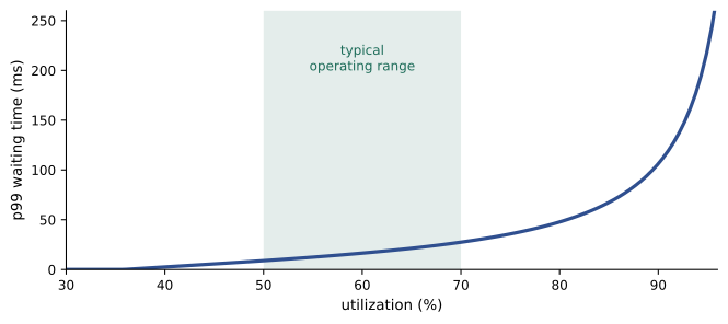
Requests arrive at random, not evenly spaced. When several arrive close together, some must wait for a free worker, and the waiting time grows sharply as the server approaches full utilization. Queueing theory describes this. The M/M/c model treats arrivals as random (Poisson) and service times as exponential, with c identical replicas; the Erlang C formula gives the probability that a request must wait, and from it the distribution of waiting times.

import math

# Queueing at a model server: c replicas, each serving one request at a time (M/M/c)
def erlang_c(c, a):
    # probability an arriving request must wait; a = offered load in replicas (lambda / mu)
    s = sum(a**k / math.factorial(k) for k in range(c))
    top = a**c / math.factorial(c) * c / (c - a)
    return top / (s + top)

service_ms = 20.0                  # mean model execution time per request
mu = 1000 / service_ms             # requests per second per replica
c = 8
print(f"{c} replicas, mean service {service_ms:.0f} ms, capacity {c * mu:.0f} requests/s")
for util in (0.5, 0.7, 0.8, 0.9, 0.95):
    lam = util * c * mu
    pw = erlang_c(c, lam / mu)
    rate = c * mu - lam                         # decay rate of waiting time, per second
    p99_wait = max(0.0, math.log(pw / 0.01) / rate * 1000) if pw > 0.01 else 0.0
    mean_wait = pw / rate * 1000
    print(f"  utilization {util:.0%}: P(wait) {pw:.2f}, mean wait {mean_wait:5.1f} ms, "
          f"p99 wait {p99_wait:6.1f} ms")

# Little law: requests in the system = arrival rate x time in system
lam = 0.8 * c * mu
print(f"At 80 % utilization, about {lam * (service_ms + 1000 * erlang_c(c, lam / mu) / (c * mu - lam)) / 1000:.1f} requests are in the system on average")

8 replicas, mean service 20 ms, capacity 400 requests/s
  utilization 50%: P(wait) 0.06, mean wait   0.3 ms, p99 wait    8.9 ms
  utilization 70%: P(wait) 0.27, mean wait   2.3 ms, p99 wait   27.5 ms
  utilization 80%: P(wait) 0.46, mean wait   5.7 ms, p99 wait   47.8 ms
  utilization 90%: P(wait) 0.70, mean wait  17.5 ms, p99 wait  106.3 ms
  utilization 95%: P(wait) 0.84, mean wait  42.2 ms, p99 wait  221.8 ms
At 80 % utilization, about 8.2 requests are in the system on average

At 50 % utilization, waiting is negligible: the p99 wait is under 10 ms. At 80 %, almost half of requests wait and the p99 wait is nearly 50 ms, more than twice the service time. At 95 %, the p99 wait exceeds 200 ms. Average latency rises only modestly, but the tail explodes, which is why model services are typically run well below full utilization, often at 50 to 70 %, with autoscaling adding capacity before the steep part of the curve. Real services differ from the idealized model (service times are less variable, traffic bursts are worse), but the shape of the curve is universal.

A related and very useful relationship is Little's law: the average number of requests in a system equals the arrival rate times the average time each spends in it.

At 320 requests per second and about 26 ms in the system, about 8 requests are in progress or waiting at any moment. Little's law helps size concurrency limits, connection pools and memory, and it holds for any stable system regardless of distributions.

Batching

Hardware such as GPUs is far more efficient processing many inputs together than one at a time, because a single input leaves most of the parallel compute idle. Batch inference exploits this. For offline jobs, large batches are simple. For online serving, dynamic batching collects requests that arrive within a short window (for example up to 5 ms, or until 32 requests are waiting) and runs them as one batch. Throughput rises dramatically, but each request may wait for the window to fill, adding latency. The batch size and window are tuned against the latency budget: at high traffic, batches fill quickly and add little delay; at low traffic, the maximum wait dominates. Model servers such as Triton and TorchServe implement dynamic batching, and language model servers use continuous batching, which adds new requests to a running batch at every generation step (AI-410, Lesson 8).

Autoscaling

Traffic varies by hour, day and season, and running enough replicas for the peak all the time wastes money. Autoscalers add and remove replicas based on a metric: CPU or GPU utilization, requests per second per replica, queue length or latency. The Kubernetes Horizontal Pod Autoscaler and serverless platforms (Knative, cloud functions, managed endpoints) are common tools. Three practical issues dominate. First, scaling takes time: starting a replica means scheduling a machine, pulling an image and loading a model, which can take minutes for large models on GPUs, so autoscalers must act before latency degrades, often with predictive schedules for known daily peaks. Second, scale-to-zero saves money for rarely used models but makes the first request after idle very slow (a cold start). Third, a minimum number of replicas spread across zones is needed for redundancy, whatever the traffic.

Caching and precomputation

If the same inputs recur, their predictions can be cached. Recommendation systems often precompute candidate lists in batch and use the online model only to rerank a few hundred candidates; search systems cache results for popular queries; embedding services cache embeddings for frequent items. Caches need expiry policies so that stale predictions are refreshed, and they change the traffic a model sees, which matters for monitoring. A hybrid of batch precomputation and lightweight online adjustment is one of the most effective serving designs.

Hardware and model efficiency

Many tabular models, such as gradient boosted trees and logistic regression, run in well under a millisecond on CPUs, and GPUs bring no benefit. Deep networks for images, audio and text usually need GPUs or other accelerators to meet latency and cost targets. Between the two, techniques that make models cheaper to run include quantization (storing weights in 8-bit or 4-bit integers instead of 32-bit floats), distillation (training a small model to imitate a large one), pruning, and compilation with runtimes such as ONNX Runtime or TensorRT that fuse operations for specific hardware. Each must be checked for accuracy loss with the tests of Lesson 4, because a faster model that is noticeably worse is not an improvement.

Load testing

Serving performance must be measured, not assumed. Load tests send realistic traffic, with the real mix of input sizes and request patterns, at increasing rates and record latency percentiles, throughput, errors and resource use. They find the rate at which the SLO is breached, show how the service behaves when overloaded (does it shed load gracefully or collapse?), and validate autoscaling. Tools such as Locust, k6 and vendor benchmarking tools make this routine; load tests should run before every major release and whenever the model or hardware changes.

Results should be compared with the latency budget at realistic traffic peaks, not just average days, since capacity must cover the busiest hour of the busiest season.