
AI-420 · Lesson 1 of 12 · 25 min
From notebook to production
A model that scores well in a notebook is the beginning of a machine learning project, not the end. To deliver value, the model must run inside a product or a business process, on fresh data, at the speed and cost the business can accept, and it must keep working as the world changes around it. Most of the effort, and most of the failures, in real machine learning projects happen in this transition from experiment to production. This course is about machine learning systems: the data pipelines, training infrastructure, deployment, serving, monitoring, testing and organizational practices, collectively called MLOps, that turn models into dependable services. This first lesson describes what an ML system contains, why ML systems are harder to run than ordinary software, the lifecycle and roles involved, and how organizations mature in their practice.
The model is a small part of the system
A widely cited paper from Google engineers, "Hidden Technical Debt in Machine Learning Systems" (Sculley and colleagues, 2015), included a diagram in which the model code was a tiny box surrounded by much larger boxes: data collection, data verification, feature extraction, configuration, resource management, serving infrastructure, monitoring, and analysis tools. The point holds a decade later. In a production recommendation, fraud detection or forecasting system, the code that defines and trains the model is often a few percent of the total. The rest moves, checks, transforms and stores data, schedules and tracks training runs, packages and serves models, and watches their behaviour.
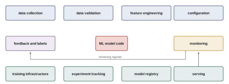
Why ML systems are different
Ordinary software encodes behaviour in code that engineers write and review. A machine learning system learns its behaviour from data, which changes several things:
- Behaviour depends on data as well as code. The same code trained on different data produces a different system, so data must be versioned, validated and tested like code.
- Failures are often silent. A bug in conventional software usually raises an error; a bug in an ML pipeline, such as a feature computed differently in training and serving, typically produces plausible but worse predictions with no error at all.
- Performance decays. The world the model was trained on drifts: customer behaviour changes, fraudsters adapt, sensors are replaced. A model that is never retrained becomes steadily less accurate.
- Testing is statistical. There is rarely a single correct output to compare against, so tests check distributions, aggregate metrics and behaviour on slices of data rather than exact values.
- Entanglement. Changing one input feature, one hyperparameter or one data source can change everything the model does, an effect Sculley and colleagues called CACE: changing anything changes everything.
- Feedback loops. A model's predictions can influence the data it will later be trained on. A recommender that shows only popular items will collect clicks only on popular items, reinforcing its own choices.
A silent failure
The most common production bug in ML systems is training-serving skew: a difference between how features are computed during training and how they are computed when the model serves predictions. Training pipelines are often batch jobs written in SQL or Spark by one team, while serving code is written in a different language by another team for low latency. Any difference, whether a unit conversion, a default value for missing data, a time zone, or a different tokenizer version, changes the inputs the model sees.
import numpy as np
from sklearn.linear_model import LogisticRegression

# Training-serving skew: the same feature computed two different ways
rng = np.random.default_rng(0)
n = 20000
spend_cents = rng.gamma(2.0, 4000, n)                 # monthly spend in cents
visits = rng.poisson(6, n)
logit = 0.0003 * spend_cents / 100 * 10 - 0.25 * visits + 0.5
churn = rng.random(n) < 1 / (1 + np.exp(-logit))

# Training pipeline (batch SQL job): spend in dollars
X_train = np.column_stack([spend_cents / 100, visits])
model = LogisticRegression().fit(X_train[:15000], churn[:15000])

test = slice(15000, n)
X_ok = X_train[test]
X_skew = np.column_stack([spend_cents[test], visits[test]])   # serving code forgot to convert cents

for name, X in [("Features as in training", X_ok), ("Serving bug: spend in cents", X_skew)]:
    p = model.predict_proba(X)[:, 1]
    acc = ((p > 0.5) == churn[test]).mean()
    print(f"{name:<30} accuracy {acc:.3f}, predicted churn rate {(p > 0.5).mean():.3f}")
print(f"Actual churn rate in test data: {churn[test].mean():.3f}")Features as in training accuracy 0.680, predicted churn rate 0.117 Serving bug: spend in cents accuracy 0.331, predicted churn rate 0.996 Actual churn rate in test data: 0.328
The model trained correctly reaches 68 % accuracy against an actual churn rate of 33 %. When the serving code forgets to convert cents to dollars, nothing crashes: the model simply receives spend values a hundred times larger, predicts that almost every customer will churn, and accuracy collapses to 33 %. If the business acted on these predictions, it would send retention offers to every customer. The defences, covered in later lessons, are to compute features once in shared code or a feature store (Lesson 2), to test the serving path against the training path (Lesson 4), and to monitor the distribution of inputs and predictions in production (Lesson 7), where a predicted churn rate jumping from 12 % to 99.6 % would trigger an alert within minutes.
The ML lifecycle
Machine learning work follows a lifecycle that loops rather than ending:
- Problem framing: what decision will the model support, what metric defines success for the business, and is ML the right tool at all? Many problems are better solved with rules or simple statistics.
- Data: collecting, labelling, cleaning and validating data, and building features (Lesson 2).
- Experimentation: training and comparing models, tracked so that results can be reproduced (Lesson 3).
- Validation: offline evaluation, testing and review before release (Lesson 4).
- Deployment: packaging the model and releasing it safely, often gradually (Lesson 5).
- Serving: answering prediction requests at the required latency, throughput and cost (Lessons 6 and 9).
- Monitoring: watching data, predictions, business outcomes and system health (Lesson 7).
- Online evaluation: measuring the real effect with experiments (Lesson 8).
- Retraining: refreshing the model on new data, manually or automatically through pipelines (Lesson 10).
Governance runs through the whole loop: documenting models, managing risk, protecting privacy and meeting regulations (Lesson 11).
Batch and online systems
A fundamental design choice is when predictions are computed. In batch prediction, a scheduled job scores all relevant entities, such as every customer every night, and stores the results in a table that applications read. Batch systems are simple, cheap and easy to monitor, but predictions can be up to a day old and are computed for entities that may never be used. In online prediction, the model runs on request, for example when a payment is submitted, with fresh features and an answer within milliseconds. Online systems handle new entities and fast-changing context, but they need low-latency infrastructure, real-time features and careful capacity planning. Streaming systems sit between them, updating features or predictions continuously as events arrive. Many organizations start with batch prediction and move to online prediction only where freshness pays for the extra complexity.
Worked problem
Choosing batch or online
A retailer wants two models: (a) a weekly demand forecast for each of 40,000 products in 300 stores, used to plan orders; and (b) a fraud score for each online payment, needed before the payment is approved. Which serving mode suits each?
Show solution
- Demand forecast: decisions are made weekly, all product-store combinations are needed, and nothing is lost by computing them in advance. Batch prediction for 12 million combinations, run overnight, fits well.
- Fraud score: each payment is new, the most useful features (amount, device, time since the last payment) exist only at the moment of payment, and the decision must be made in well under a second. This requires online prediction with real-time features.
Answer: Batch for the forecast, online for fraud. The choice follows from when the decision is made, when the input data become available, and how many predictions are actually used.
Roles and teams
Production ML involves several specialties. Data scientists frame problems, explore data and develop models. ML engineers turn models into reliable, efficient software and build training and serving pipelines. Data engineers build and maintain the pipelines that collect and transform data. Platform or MLOps engineers build shared infrastructure: feature stores, experiment tracking, model registries, deployment and monitoring tools. Product managers and domain experts define what success means, and risk, privacy and legal specialists review models with significant effects on people. Small teams combine these roles; large organizations separate them, which brings the risk that each team optimizes its own part and no one owns the whole system. Clear ownership of each production model, including who is paged when it misbehaves, is one of the most important organizational decisions.
MLOps maturity
MLOps borrows from DevOps the idea of automating the path from change to production, adding the extra dimensions of data and models. Organizations often describe their maturity in levels. At level 0, everything is manual: a data scientist trains a model in a notebook and hands a file to engineers, who deploy it; retraining is rare and painful. At level 1, the training pipeline is automated, so that models can be retrained on new data with the same code, and models are tracked in a registry. At level 2, the pipelines themselves are built, tested and deployed automatically through continuous integration and delivery, and retraining is triggered by schedules or monitoring signals. Not every model needs level 2; the right level depends on how often the data change, how many models there are, and how costly errors are. But level 0 rarely survives contact with a model that matters.
| Level | Training | Deployment | Retraining |
|---|---|---|---|
| 0: manual | Notebook, by hand | Model file handed over | Rare, manual |
| 1: pipeline automation | Automated pipeline | Registry, scripted release | Scheduled or on demand |
| 2: CI/CD for pipelines | Pipelines tested and deployed automatically | Gradual, automated rollout | Triggered by schedule or monitoring |
How this course is organized
The section at the end of the lesson shows how the twelve lessons fit together.
- Lesson 1 (this lesson): from notebook to production.
- Lesson 2: data pipelines, validation and feature stores.
- Lesson 3: experiment tracking, reproducibility and model registries.
- Lesson 4: testing machine learning systems.
- Lesson 5: packaging and deployment patterns.
- Lesson 6: model serving, latency and throughput.
- Lesson 7: monitoring, drift and retraining.
- Lesson 8: online experiments and A/B testing.
- Lesson 9: cost and infrastructure.
- Lesson 10: pipelines, orchestration and continuous training.
- Lesson 11: reliability, security and governance.
- Lesson 12: case study and capstone project.
The course assumes you can train and evaluate models (AI-220) and write and test software (CMPUT-301). Examples use Python with NumPy, pandas and scikit-learn, and describe widely used open-source tools such as MLflow, Airflow, Kubernetes and Prometheus without depending on any one product.
Common mistakes
MistakeTreating a good notebook score as a finished project.
InsteadPlan for data pipelines, serving, monitoring and retraining from the start.
MistakeComputing features separately in training and serving code.
InsteadShare feature code or use a feature store, and test for skew.
MistakeAssuming a deployed model keeps its accuracy.
InsteadMonitor for drift and plan retraining.
MistakeChoosing online serving by default.
InsteadUse batch prediction unless freshness justifies the complexity.
MistakeLeaving production models without a clear owner.
InsteadAssign ownership, including who responds when a model misbehaves.
Summary and key terms
- Model code is a small part of a production ML system.
- ML behaviour depends on data; failures are often silent and performance decays.
- Training-serving skew is the most common silent failure.
- The lifecycle loops from framing through data, experiments, deployment, monitoring and retraining.
- Batch prediction is simple and cheap; online prediction gives freshness at higher complexity.
- Production ML needs several roles and clear model ownership.
- MLOps maturity runs from manual work to automated, tested pipelines.
- MLOps
- Practices and tools for deploying and maintaining ML systems reliably.
- Technical debt
- The future cost of shortcuts taken in building a system.
- Training-serving skew
- A difference between features in training and in serving.
- Drift
- Change over time in the data or relationships a model depends on.
- CACE
- Changing anything changes everything: entanglement in ML systems.
- Feedback loop
- Predictions influencing the data later used for training.
- Batch prediction
- Scoring entities on a schedule and storing the results.
- Online prediction
- Scoring each request when it arrives.
- Model registry
- A catalogue of trained models, versions and their status.
- Maturity level
- A description of how automated an organization's ML practice is.
Practice problems
Work each problem on paper first, then reveal the answer to check.
Why is the model only a small part of a production ML system?
Show answer
Most code handles data collection, validation, features, configuration, infrastructure, serving and monitoring.
Give three ways ML systems differ from ordinary software.
Show answer
For example: behaviour depends on data, failures are silent, performance decays, testing is statistical, entanglement, feedback loops.
What is training-serving skew?
Show answer
A difference between how features are computed in training and in serving.
From the output, what happened to accuracy and predicted churn when spend was in cents?
Show answer
Accuracy fell from 0.680 to 0.331 and predicted churn rose from 11.7 % to 99.6 %.
Why did no error appear in the skew example?
Show answer
The inputs were valid numbers; only their scale was wrong.
What monitoring signal would have caught the skew bug quickly?
Show answer
The input spend distribution or the predicted churn rate shifting sharply.
Give one advantage and one drawback of batch prediction.
Show answer
Simple and cheap; predictions can be stale and computed for unused entities.
Why does a fraud model need online prediction?
Show answer
The key features exist only at payment time and the decision is needed within a second.
What is a feedback loop in a recommender?
Show answer
Showing only some items means clicks are collected only on those items, reinforcing the model's choices.
What distinguishes MLOps maturity level 1 from level 0?
Show answer
The training pipeline is automated and models are tracked in a registry.
Lesson quiz · 5 questions
Score 60% or more to complete this lesson.
Create a free account to save your progress, take quizzes and earn a certificate.