Scaling laws

Training a frontier language model costs tens to hundreds of millions of dollars in compute, so organizations need to predict, before spending it, how good a model will be and how to divide a budget between model size and training data. Scaling laws make this possible. They are empirical relationships, measured across many training runs, showing that a model's loss falls smoothly and predictably as parameters, data and compute increase. This lesson explains power laws, the original OpenAI scaling laws, the compute-optimal "Chinchilla" result, why practical models are often trained far beyond that optimum, the debate over emergent abilities, the limits posed by data, and the newer scaling of compute at inference time.

Power laws

A power law has the form \(y = a x^{-b}\). Taking logarithms gives \(\log y = \log a - b \log x\), a straight line on a log-log plot with slope \(-b\). Power laws describe many phenomena where there is no characteristic scale: each tenfold increase in \(x\) reduces \(y\) by the same factor \(10^{-b}\).

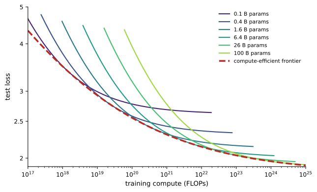
In 2020, researchers at OpenAI (Kaplan and colleagues) trained hundreds of transformer language models of different sizes on different amounts of data and found that test loss followed power laws in each of three quantities when the others were not limiting: parameters \(N\), dataset size \(D\), and compute \(C\). The trends held across more than six orders of magnitude, and architectural details such as depth versus width mattered much less than total scale.

with exponents around 0.07 to 0.10 in their setup. Small exponents mean that each tenfold increase in scale reduces loss by a modest but reliable fraction, which is why progress has required exponential growth in compute.

Irreducible loss and the combined law

Loss cannot fall to zero: natural text contains genuine uncertainty (what word an author chose, what comes next in a conversation). A better functional form includes an irreducible term \(E\), the entropy of the text, plus separate terms for the limits imposed by finite parameters and finite data:

This form, introduced in DeepMind's 2022 Chinchilla paper, says that a model is limited both by its size and by how much data it has seen. Fitting it requires care: a pure power law fitted to small models without the irreducible term can badly mislead when extrapolated.

import numpy as np

rng = np.random.default_rng(0)
N = np.array([1e7, 3e7, 1e8, 3e8, 1e9])
true = lambda n: 1.8 + 480 / n ** 0.35
L = true(N) * (1 + rng.normal(0, 0.005, N.size))

b, log_a = np.polyfit(np.log(N), np.log(L), 1)
print(f"pure power law fit: L = {np.exp(log_a):.2f} * N^({b:.3f})")

best = None
for E in np.linspace(0.5, 2.5, 401):
    if E >= L.min():
        break
    s, c = np.polyfit(np.log(N), np.log(L - E), 1)
    err = np.sum((E + np.exp(c) * N ** s - L) ** 2)
    if best is None or err < best[0]:
        best = (err, E, s, c)
_, E, s, c = best
print(f"with irreducible term: L = {E:.2f} + {np.exp(c):.0f} * N^({s:.3f})")
for n in [1e10, 1e11]:
    p1 = np.exp(log_a) * n ** b
    p2 = E + np.exp(c) * n ** s
    print(f"N={n:.0e}  true {true(n):.3f}  pure power law {p1:.3f}  with E {p2:.3f}")

pure power law fit: L = 19.08 * N^(-0.107)
with irreducible term: L = 1.78 + 419 * N^(-0.341)
N=1e+10  true 1.952  pure power law 1.617  with E 1.939
N=1e+11  true 1.868  pure power law 1.263  with E 1.850

The pure power law fits the five points but predicts losses that keep falling steeply, missing the floor that the true curve approaches. The form with an irreducible term extrapolates far better. Scaling-law practice involves exactly this kind of fitting on small runs, then checking predictions against a few larger runs before committing the full budget.

Compute-optimal training: Chinchilla

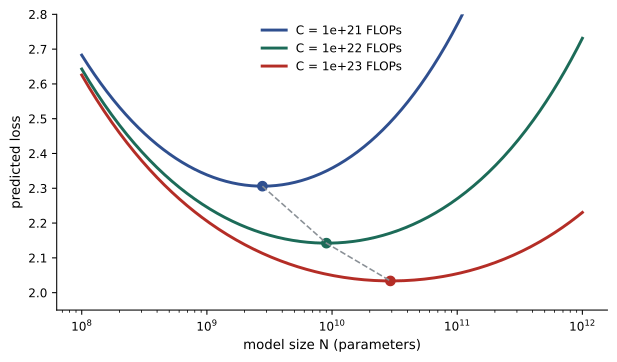
Given a fixed compute budget \(C \approx 6ND\), should you train a larger model on fewer tokens or a smaller model on more tokens? The 2020 OpenAI analysis suggested putting most extra compute into larger models, and models such as GPT-3 (175 billion parameters, about 300 billion tokens) followed that advice. In 2022, DeepMind's Hoffmann and colleagues trained over 400 models and concluded that parameters and tokens should grow in roughly equal proportion with compute, which works out to about 20 training tokens per parameter.

They demonstrated this with Chinchilla, a 70-billion-parameter model trained on 1.4 trillion tokens. It used about the same compute as their earlier 280-billion-parameter Gopher model (trained on 300 billion tokens) but outperformed it on most benchmarks, and being four times smaller it was also cheaper to use. A 2024 replication by Epoch AI corrected the paper's fitted constants for the parametric loss function, giving values close to \(E = 1.82\), \(A = 482\), \(B = 2085\), \(\alpha = 0.35\), \(\beta = 0.37\), consistent with the roughly 20-to-1 rule.

import numpy as np

E, A, B, alpha, beta = 1.82, 482.0, 2085.4, 0.348, 0.366


def loss(N, D):
    return E + A / N ** alpha + B / D ** beta


for C in [1e20, 1e21, 1e22, 1e23, 1e24]:
    N = np.logspace(7, 13, 4000)
    D = C / (6 * N)
    L = loss(N, D)
    i = int(np.argmin(L))
    print(f"C={C:.0e}  best N={N[i] / 1e9:7.2f}B  D={D[i] / 1e9:8.0f}B  tokens/param={D[i] / N[i]:5.1f}  loss={L[i]:.3f}")

C = 5.8e23
for N in [70e9, 280e9, 530e9]:
    D = C / (6 * N)
    print(f"same compute, N={N / 1e9:4.0f}B  D={D / 1e9:5.0f}B  loss={loss(N, D):.3f}")

C=1e+20  best N=   0.85B  D=      20B  tokens/param= 22.9  loss=2.553
C=1e+21  best N=   2.78B  D=      60B  tokens/param= 21.6  loss=2.306
C=1e+22  best N=   9.06B  D=     184B  tokens/param= 20.3  loss=2.142
C=1e+23  best N=  29.44B  D=     566B  tokens/param= 19.2  loss=2.034
C=1e+24  best N=  95.94B  D=    1737B  tokens/param= 18.1  loss=1.962
same compute, N=  70B  D= 1381B  loss=1.976
same compute, N= 280B  D=  345B  loss=1.995
same compute, N= 530B  D=  182B  loss=2.018

Beyond compute-optimal: training for inference

Chinchilla optimality minimizes the cost of training for a given loss. But a model that will serve billions of requests also incurs inference costs, which grow with model size. Training a smaller model on far more tokens than the 20-to-1 rule costs more training compute for the same loss, but gives a model that is cheaper to run for its whole life. Since 2023, many widely used models have been trained this way: Meta's Llama 3 8B model, for example, was trained on about 15 trillion tokens, nearly 1,900 tokens per parameter. Loss continues to improve with more tokens, only more slowly than the compute-optimal path. Small models trained long, often with distillation from larger "teacher" models, now power many on-device and low-cost applications.

Scaling, capabilities and emergence

Loss falls smoothly, but what users care about is capabilities: answering questions correctly, writing working code, solving problems. Benchmark accuracy also tends to improve with scale, and some capabilities have appeared to emerge suddenly, near zero for smaller models and then rising sharply above some size, an observation reported widely in 2022. A 2023 analysis by Schaeffer and colleagues argued that many apparent jumps are artefacts of the metrics used: an all-or-nothing score such as exact match of a multi-step answer rises abruptly even when the underlying probability of each step improves smoothly. With continuous metrics the trends are usually smooth. Predicting specific capabilities remains harder than predicting loss, which is one reason labs evaluate models extensively for both useful and dangerous capabilities as they scale.

The data constraint

Compute-optimal scaling requires ever more training tokens, but the supply of high-quality human-written text is finite. Estimates suggest that the stock of public, high-quality text is in the hundreds of trillions of tokens, a limit that frontier training could approach within a few years. Responses include:

• Repeating data: experiments (Muennighoff and colleagues, 2023) found that repeating a dataset for up to about four epochs gives almost the same benefit as fresh data, with diminishing returns after that.
• Better filtering: extracting more value from each token through quality selection.
• Synthetic data: text, code and reasoning traces generated by models, verified where possible (for example by running code or checking math answers). Training only on unverified model outputs can cause model collapse, a gradual loss of diversity and accuracy.
• Multimodal data: images, audio and video add very large data sources.
• Licensed and private data: books, news archives and specialized data obtained through agreements.

Scaling inference-time compute

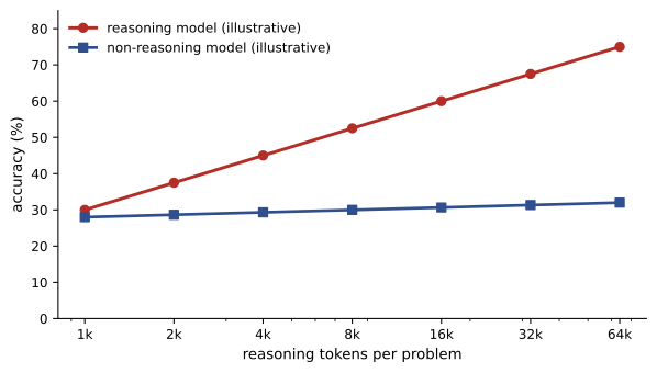
Since 2024, a second scaling axis has become central: compute spent while answering. Reasoning models, starting with OpenAI's o1 (September 2024) and followed by DeepSeek-R1 (January 2025) and reasoning modes in other model families, are trained with reinforcement learning to produce long chains of intermediate reasoning before answering (Lesson 5). Their accuracy on math, science and coding problems rises smoothly with the number of reasoning tokens they are allowed to generate, roughly log-linearly, much as training loss improves with training compute. Other forms of test-time scaling include sampling many answers and choosing by majority vote or a verifier. This makes inference infrastructure, latency and cost an even larger part of the economics of AI (DCE-410).

Lesson 4 looks at the other half of the scaling equation, the training data itself: where it comes from, how it is filtered and deduplicated, and what happens as high-quality text runs short.