Pretraining language models at scale

Large language models (LLMs) such as the systems behind Claude, ChatGPT, Gemini, Llama and DeepSeek are neural networks trained to predict the next piece of text. That simple objective, applied to trillions of words with networks of billions to trillions of parameters, produces systems that can write, summarize, translate, reason through problems, write code and hold conversations. This course explains how such models are built, evaluated and used, from pretraining (this lesson) to building complete applications (Lesson 12), and the section at the end of this lesson shows how the twelve lessons fit together. It builds on the transformer and attention material in AI-340.

From next-token prediction to general capability

A language model assigns probabilities to sequences of tokens (pieces of text). By the chain rule of probability, the probability of a sequence is the product of the probabilities of each token given the ones before it:

Pretraining fits a model to maximize this probability on a huge corpus, or equivalently to minimize the cross-entropy loss, the average negative log probability the model assigns to each actual next token:

Why does next-token prediction produce general abilities? To predict text well, a model must capture everything that makes text predictable: grammar, facts about the world, the structure of arguments, the conventions of code, the way characters in a story behave, and the steps of a worked solution. Pretraining is thus a form of self-supervised learning: the labels (the next tokens) come free with the data, so the model can learn from essentially all the text that can be collected.

Loss is often reported as perplexity, the exponential of the cross-entropy, which can be read as the effective number of equally likely choices the model is uncertain between at each step. Lower is better. When loss is measured in bits (base-2 logarithms), perplexity is \(2^{\mathcal{L}}\).

import numpy as np

train = "the cat sat on the mat. the dog sat on the log. a cat and a dog met on the mat. " * 20
test = "the dog sat on the mat. a cat met the dog."
chars = sorted(set(train + test))
ix = {c: i for i, c in enumerate(chars)}
V = len(chars)


def fit(text, k):
    counts = np.full((V, V), k)
    for a, b in zip(text, text[1:]):
        counts[ix[a], ix[b]] += 1
    return counts / counts.sum(axis=1, keepdims=True)


def cross_entropy(P, text):
    logp = [np.log2(P[ix[a], ix[b]]) for a, b in zip(text, text[1:])]
    return -float(np.mean(logp))


print("vocabulary size:", V, " uniform guess:", round(float(np.log2(V)), 2), "bits/char")
for k in [0.01, 0.1, 1.0]:
    P = fit(train, k)
    h_tr, h_te = cross_entropy(P, train), cross_entropy(P, test)
    print(f"smoothing {k:<4}  train {h_tr:.2f} bits/char  test {h_te:.2f} bits/char  test perplexity {2 ** h_te:.2f}")
P = fit(train, 0.1)
row = P[ix["t"]]
top = np.argsort(row)[::-1][:3]
print("after t:", [(chars[i], round(float(row[i]), 2)) for i in top])

vocabulary size: 14  uniform guess: 3.81 bits/char
smoothing 0.01  train 1.38 bits/char  test 1.35 bits/char  test perplexity 2.55
smoothing 0.1   train 1.40 bits/char  test 1.36 bits/char  test perplexity 2.57
smoothing 1.0   train 1.52 bits/char  test 1.48 bits/char  test perplexity 2.79
after t: [(' ', 0.41), ('h', 0.41), ('.', 0.17)]

The bigram model in the code predicts each character from only the previous one, reaching about 1.4 bits per character on this tiny repetitive text. Modern LLMs condition on thousands to millions of previous tokens through attention, which is what lets them use context, follow instructions and maintain coherence over long documents.

Tokenization

Models operate on tokens rather than characters or whole words. Most LLMs use subword tokenizers built with byte-pair encoding (BPE) or similar algorithms. BPE starts with individual bytes or characters and repeatedly merges the most frequent adjacent pair into a new token, until the vocabulary reaches a target size (commonly 32,000 to over 200,000 tokens). Frequent words become single tokens; rare words are split into pieces; any text can be represented, because the base alphabet covers all bytes.

from collections import Counter

corpus = ["low", "lower", "lowest", "newer", "newest", "wider", "widest", "new", "low", "newest"]
words = Counter(tuple(w) + ("_",) for w in corpus)


def pair_counts(words):
    pairs = Counter()
    for w, n in words.items():
        for a, b in zip(w, w[1:]):
            pairs[(a, b)] += n
    return pairs


def merge(words, pair):
    out = Counter()
    for w, n in words.items():
        new, i = [], 0
        while i < len(w):
            if i < len(w) - 1 and (w[i], w[i + 1]) == pair:
                new.append(w[i] + w[i + 1]); i += 2
            else:
                new.append(w[i]); i += 1
        out[tuple(new)] += n
    return out


merges = []
for step in range(8):
    pairs = pair_counts(words)
    best = max(pairs, key=lambda p: (pairs[p], p))
    merges.append(best)
    words = merge(words, best)
    print(f"merge {step + 1}: {best[0]} + {best[1]} -> {best[0] + best[1]}  (count {pairs[best]})")


def encode(word):
    w = tuple(word) + ("_",)
    for p in merges:
        w = tuple(merge(Counter({w: 1}), p))[0]
    return list(w)


for w in ["lowest", "newer", "slower"]:
    print(w, "->", encode(w))

merge 1: w + e -> we  (count 5)
merge 2: t + _ -> t_  (count 4)
merge 3: s + t_ -> st_  (count 4)
merge 4: n + e -> ne  (count 4)
merge 5: l + o -> lo  (count 4)
merge 6: we + st_ -> west_  (count 3)
merge 7: w + _ -> w_  (count 3)
merge 8: r + _ -> r_  (count 3)
lowest -> ['lo', 'west_']
newer -> ['ne', 'we', 'r_']
slower -> ['s', 'lo', 'we', 'r_']

Tokenization has practical consequences. English text averages roughly three quarters of a word per token, while many other languages, code and numbers use more tokens per word, making them more expensive to process and sometimes less well modelled. Arithmetic and spelling tasks can be harder because numbers and words are split into irregular pieces. Context window limits and API prices are measured in tokens.

The model: a decoder-only transformer

Almost all current LLMs are decoder-only transformers (AI-340). Each token is mapped to an embedding vector; a stack of identical blocks then transforms the sequence of vectors. Each block contains a causal self-attention layer, which lets each position gather information from earlier positions (but not later ones, so the model cannot peek at the token it must predict), and a feed-forward network applied to each position, with residual connections and normalization around both. A final layer maps each position's vector to logits over the vocabulary, and a softmax gives the next-token probabilities.

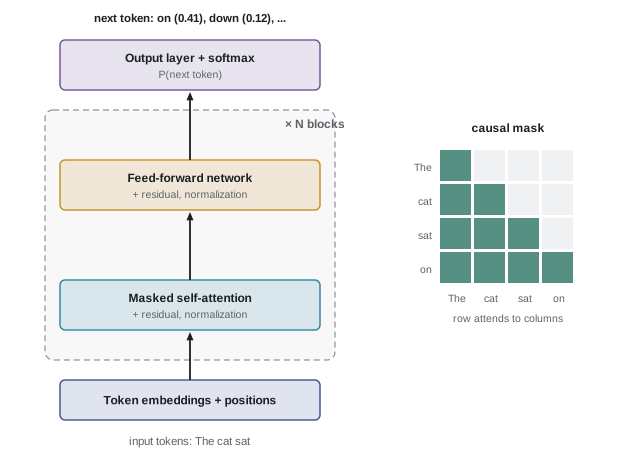
Modern models add refinements: rotary position embeddings for relative positions, grouped-query attention to shrink memory use during generation, gated feed-forward layers (such as SwiGLU), pre-normalization for stable training, and often mixture-of-experts (MoE) layers. An MoE layer contains many feed-forward "experts" and a router that sends each token to only a few of them, so the total number of parameters can be very large while the computation per token stays moderate. Several leading open-weight models released since 2024, such as DeepSeek-V3 and Llama 4, use mixture-of-experts.

The parameter count of a standard (dense) transformer is dominated by its blocks. With \(L\) layers and model width \(d\), each block has about \(4d^2\) attention parameters and \(8d^2\) feed-forward parameters (for a feed-forward width of \(4d\)), giving roughly:

where \(V d\) counts the token embeddings for a vocabulary of size \(V\).

Training compute

The compute needed to train a dense transformer is well approximated by a simple rule: each parameter is used in about 2 floating-point operations (FLOPs) per token in the forward pass and about 4 in the backward pass, so:

where \(C\) is total training FLOPs, \(N\) the number of parameters and \(D\) the number of training tokens. Training runs are carried out on clusters of thousands to hundreds of thousands of GPUs or other accelerators (DCE-410 covers the facilities). The fraction of the hardware's peak throughput actually achieved, called model FLOPs utilization (MFU), is typically 30% to 50% for large runs.

def params(layers, d_model, vocab):
    blocks = 12 * layers * d_model ** 2
    embed = vocab * d_model
    return blocks, embed


configs = [("small", 12, 768, 50000), ("medium", 24, 2048, 50000), ("large", 32, 4096, 128000), ("x-large", 80, 8192, 128000)]
peak = 989e12
mfu = 0.40
for name, L, d, V in configs:
    blocks, embed = params(L, d, V)
    N = blocks + embed
    D = 20 * N
    C = 6 * N * D
    gpu_hours = C / (peak * mfu) / 3600
    mem_gb = 16 * N / 1e9
    print(f"{name:<8} N={N / 1e9:6.2f}B  D={D / 1e9:7.0f}B tokens  C={C:.1e}  GPU-h={gpu_hours:9,.0f}  state={mem_gb:5.0f} GB")

small    N=  0.12B  D=      2B tokens  C=1.8e+18  GPU-h=        1  state=    2 GB
medium   N=  1.31B  D=     26B tokens  C=2.1e+20  GPU-h=      145  state=   21 GB
large    N=  6.97B  D=    139B tokens  C=5.8e+21  GPU-h=    4,090  state=  111 GB
x-large  N= 65.47B  D=   1309B tokens  C=5.1e+23  GPU-h=  361,200  state= 1048 GB

Memory is the other constraint. During training with the Adam optimizer in mixed precision, each parameter needs roughly 16 bytes (weights, gradients and two optimizer moments, some in 32-bit precision), plus memory for activations. A 70-billion-parameter model therefore needs over a terabyte for its training state alone, far more than one GPU holds. Training is distributed using several forms of parallelism together:

• Data parallelism: each group of GPUs processes different batches and averages gradients; sharded variants (such as ZeRO or FSDP) also split optimizer state and weights across GPUs.
• Tensor parallelism: individual matrix multiplications are split across GPUs within a server.
• Pipeline parallelism: different layers run on different GPUs, with micro-batches flowing through like an assembly line.
• Expert parallelism: in mixture-of-experts models, different experts live on different GPUs.

Pretraining data

Pretraining corpora contain trillions of tokens drawn from web pages (often starting from Common Crawl), books, scientific papers, code repositories, encyclopedias, forums and, increasingly, synthetic data generated by other models. Raw web text is noisy, so data pipelines invest heavily in:

• Extraction: pulling clean text from HTML.
• Language identification and filtering.
• Quality filtering: heuristics and classifiers that keep educational, well-written text and remove spam, boilerplate and machine-generated junk.
• Deduplication: removing exact and near-duplicate documents, which otherwise waste compute and encourage memorization.
• Safety and privacy filtering: removing personal information, toxic content and material that should not be learned.
• Decontamination: removing copies of benchmark test sets so that evaluations remain meaningful.
• Mixing: choosing proportions of web, code, math, books and other sources, often changing them during training (for example, more high-quality data near the end).

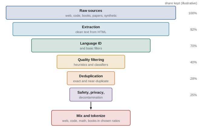
Data quality matters as much as quantity: carefully filtered datasets let smaller models match larger ones trained on raw web text. Where the data comes from also raises legal and ethical questions about copyright, consent and attribution, discussed in Lesson 9.

The training run

A pretraining run is planned around a fixed compute budget. Engineers choose the model size and number of tokens (Lesson 3), the learning rate schedule (usually a warm-up followed by cosine or step decay, or a constant rate with a final cooldown), the batch size (often millions of tokens per step), and the context length (often trained short first and extended later). They run many small experiments to choose hyperparameters, then monitor the main run for loss spikes and divergence, which can be caused by bad data, numerical instability or hardware faults, and roll back to a checkpoint when necessary. Evaluations on held-out data and benchmarks are run throughout.

The result of pretraining is a base model: a powerful text predictor that continues whatever text it is given. It has broad knowledge and skills, but it does not reliably follow instructions, may continue a question with more questions, and reflects the biases and errors of its data. Lesson 5 describes how post-training turns a base model into an assistant.

How this course is organized

The twelve lessons follow a language model from its construction to its use in real applications:

• Lesson 1 (this lesson): pretraining, tokenization, architecture and training compute.
• Lesson 2: attention, position encoding, the KV cache and long context.
• Lesson 3: scaling laws and compute-optimal training.
• Lesson 4: data for language models: filtering, deduplication, mixtures, synthetic data and contamination.
• Lesson 5: fine-tuning and learning from human feedback.
• Lesson 6: evaluating language models.
• Lesson 7: prompting, retrieval and tool use.
• Lesson 8: efficient inference and serving.
• Lesson 9: diffusion and multimodal models.
• Lesson 10: embeddings, contrastive learning and vector search.
• Lesson 11: safety, misuse and responsible deployment.
• Lesson 12: building language model applications, with a course project.