
AI-340 · Lesson 7 of 12 · 25 min
Pretrained language models and scaling
Until about 2018, most NLP systems were trained from scratch for each task on labelled data, with perhaps pretrained word embeddings (Lesson 2) as input. The transformer (Lesson 6) made a different approach practical: pretrain a large model on vast amounts of unlabelled text with a self-supervised objective, then adapt it to many tasks. This transfer learning approach transformed the field within two years and led directly to today's large language models. This lesson explains the three main families of pretrained models (encoders such as BERT, decoders such as GPT, and encoder-decoders such as T5), their pretraining objectives, how they are adapted to tasks, the data they are trained on, and the scaling laws that relate model size, data and compute to performance.
Self-supervised pretraining
Self-supervised learning creates training targets from the text itself, so any text can be used without labels. The model is trained to predict hidden or future parts of the input, and in doing so learns syntax, word meanings, facts about the world and patterns of reasoning that turn out to be useful for many tasks. Three objectives dominate:
- Causal (autoregressive) language modelling: predict each token from the tokens before it, \(\max \sum_t \log P(x_t \mid x_{<t})\), the same objective as the n-gram models of Lesson 1. It is used by decoder-only models such as the GPT family.
- Masked language modelling: replace a random 15% of tokens with a mask symbol (or random tokens) and predict the originals from both left and right context. It is used by encoder models such as BERT.
- Span corruption (denoising): replace random spans of text with sentinel tokens and train an encoder-decoder to generate the missing spans, as in T5.
| Family | Examples | Pretraining objective | Attention | Best suited to |
|---|---|---|---|---|
| Encoder-only | BERT, RoBERTa, DeBERTa | masked language modelling | bidirectional | classification, tagging, retrieval embeddings |
| Decoder-only | GPT series, Llama, Mistral, Claude | causal language modelling | causal (left to right) | generation, chat, few-shot tasks; now general-purpose |
| Encoder-decoder | T5, BART, mT5 | span corruption or denoising | bidirectional encoder, causal decoder | translation, summarization, text-to-text tasks |
Encoders see the whole input at once, which suits understanding tasks; decoders can generate text naturally. Since around 2020, decoder-only models have become dominant because, at large scale, a single generative model can perform almost any task specified in text, while encoders remain the workhorses for efficient classification, tagging and embedding models used in search (Lesson 9).
BERT and fine-tuning
BERT (2018) was pretrained with masked language modelling on books and Wikipedia, plus a next-sentence prediction task later found unnecessary. Its input begins with a special [CLS] token, whose final hidden state summarizes the sequence, and pairs of sentences are separated by [SEP]. To adapt BERT to a task, a small output layer is added and the whole network is fine-tuned on labelled data for a few epochs: a classification layer on [CLS] for sentence classification (Lesson 3), a per-token layer for tagging, or start and end pointers for extractive question answering (Lesson 11). BERT set new records on almost every NLP benchmark of its time, often with only thousands of labelled examples, because most of the needed knowledge came from pretraining.
Successors improved the recipe: RoBERTa trained longer on more data and dropped next-sentence prediction; DeBERTa improved attention with separate content and position representations; ELECTRA replaced masked prediction with detecting which tokens were replaced by a small generator, using every token for training and learning more efficiently; and distilled models such as DistilBERT compressed BERT for faster inference (Lesson 10).
GPT and in-context learning
The GPT series took the decoder route. GPT-2 (2019) showed that a large causal language model could perform tasks such as summarization and translation without task-specific training when prompted appropriately. GPT-3 (2020), with 175 billion parameters, demonstrated in-context learning: given a few examples of a task in the prompt (few-shot prompting), the model performs the task on a new input, with no change to its weights. Performance improved steadily with scale, and abilities such as arithmetic and multi-step reasoning appeared to emerge in larger models. Subsequent work turned these pretrained models into assistants through instruction tuning and reinforcement learning from human feedback (Lesson 8).
T5 and the text-to-text framework
T5 (2019) cast every task as converting input text to output text: "translate English to French: ...", "summarize: ...", "cola sentence: ..." for grammatical acceptability, and so on, with a single encoder-decoder model and one training objective. The T5 paper also systematically compared pretraining objectives, architectures, data sets and model sizes, an influential study of what matters. Multilingual versions such as mT5 extended the approach to 101 languages.
Pretraining data
Pretrained models learn from very large text collections: web crawls such as Common Crawl, filtered and deduplicated (for example C4, RefinedWeb, FineWeb), books, Wikipedia, scientific papers, code repositories, and conversational data. Modern large models train on trillions of tokens. Data quality has proved as important as quantity:
- Filtering removes boilerplate, spam, very short or machine-generated pages, using heuristics and quality classifiers.
- Deduplication removes repeated documents and passages, which waste compute and increase memorization of training data.
- Mixtures balance web text with high-quality sources, code and multilingual data, with weights tuned by experiment.
- Safety and privacy filtering remove personal information and harmful content.
- Contamination checks ensure that evaluation benchmarks have not leaked into training data, which would inflate scores (Lesson 12).
Training data also raise legal and ethical questions about copyright, consent and compensation, which are the subject of litigation and policy debate in several countries.
Counting parameters and compute
A transformer layer with model dimension \(d\) has about \(4d^2\) parameters in its attention projections and \(8d^2\) in a feed-forward block with hidden size \(4d\), so about \(12d^2\) per layer, plus a token embedding matrix of size vocabulary × \(d\). Training a model with \(N\) parameters on \(D\) tokens takes roughly \(6ND\) floating-point operations: about \(2N\) per token for the forward pass and \(4N\) for the backward pass.
def transformer_params(layers, d, vocab, ff_mult=4):
    attn = 4 * d * d                                    # query, key, value and output projections
    ffn = 2 * ff_mult * d * d                           # two feed-forward matrices
    return layers * (attn + ffn) + vocab * d            # plus the token embedding matrix (biases and norms ignored)

models = {"BERT-base (encoder)": (12, 768, 30522), "GPT-2 small (decoder)": (12, 768, 50257), "GPT-2 XL": (48, 1600, 50257), "a 7B decoder": (32, 4096, 32000)}
for name, (L, d, V) in models.items():
    print(f"{name:22s}: about {transformer_params(L, d, V) / 1e6:7.0f} million parameters")

# Training compute and time: about 6 FLOPs per parameter per token
N, tokens = 7e9, 2e12
flops = 6 * N * tokens
gpu_flops = 400e12 * 0.40                               # a GPU at 400 TFLOP/s peak and 40% utilization
print(f"7B model on 2 trillion tokens: {flops:.1e} FLOPs = {flops / gpu_flops / 3600 / 24:,.0f} GPU-days, or {flops / gpu_flops / 3600 / 24 / 1024:.0f} days on 1,024 GPUs")BERT-base (encoder) : about 108 million parameters GPT-2 small (decoder) : about 124 million parameters GPT-2 XL : about 1555 million parameters a 7B decoder : about 6574 million parameters 7B model on 2 trillion tokens: 8.4e+22 FLOPs = 6,076 GPU-days, or 6 days on 1,024 GPUs
The approximation reproduces BERT-base (110 million) and GPT-2 small (124 million) closely; real 7B models differ in details such as gated feed-forward layers but have similar totals. Training a 7B model on 2 trillion tokens takes about \(8 \times 10^{22}\) operations, roughly a week on a thousand modern GPUs, while frontier models use 100 to 1,000 times more compute.
Scaling laws
Studies from 2020 onward found that a language model's loss on held-out text falls smoothly and predictably as a power law in model size, data size and compute, over many orders of magnitude. The Chinchilla study (2022) fitted the loss as
where \(E\) is the irreducible loss of natural text and the other terms shrink as parameters \(N\) and training tokens \(D\) grow. For a fixed compute budget \(C \approx 6ND\), the loss is minimized by scaling parameters and data roughly in proportion. The study's headline conclusion was that compute-optimal training uses about 20 tokens per parameter, far more data than earlier models such as GPT-3 had used.
import numpy as np

# Chinchilla-style loss fit: L(N, D) = E + A / N^alpha + B / D^beta (constants from Hoffmann et al., 2022)
E, A, B, alpha, beta = 1.69, 406.4, 410.7, 0.34, 0.28
loss = lambda N, D: E + A / N ** alpha + B / D ** beta

for C in (1e21, 1e23, 1e25):                            # training compute in FLOPs, using C = 6 N D
    Ns = np.logspace(7, 13, 2000)
    Ds = C / (6 * Ns)
    L = loss(Ns, Ds)
    k = np.argmin(L)
    print(f"compute {C:.0e} FLOPs: best N = {Ns[k]:.2e} parameters, D = {Ds[k]:.2e} tokens ({Ds[k] / Ns[k]:.0f} tokens per parameter), loss {L[k]:.3f}")
# A model trained on far fewer tokens than optimal for its size (similar to GPT-3)
N, D = 175e9, 300e9
C = 6 * N * D
Ns = np.logspace(9, 12, 3000)
best = Ns[np.argmin(loss(Ns, C / (6 * Ns)))]
print(f"175B parameters on 300B tokens: loss {loss(N, D):.3f}; the same compute with {best:.2e} parameters on {C / (6 * best):.2e} tokens: loss {loss(best, C / (6 * best)):.3f}")compute 1e+21 FLOPs: best N = 1.82e+09 parameters, D = 9.16e+10 tokens (50 tokens per parameter), loss 2.329 compute 1e+23 FLOPs: best N = 1.46e+10 parameters, D = 1.14e+12 tokens (78 tokens per parameter), loss 2.005 compute 1e+25 FLOPs: best N = 1.17e+11 parameters, D = 1.43e+13 tokens (122 tokens per parameter), loss 1.845 175B parameters on 300B tokens: loss 2.002; the same compute with 2.45e+10 parameters on 2.14e+12 tokens: loss 1.954
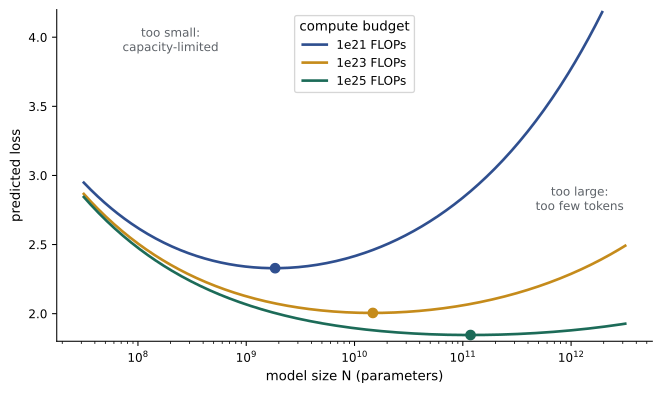
A GPT-3-like allocation (175 billion parameters on 300 billion tokens) achieves a worse loss than a model about seven times smaller trained on seven times more tokens with the same compute. The exact optimal ratio depends on how the law is fitted (this particular fit suggests more tokens per parameter at larger budgets than the 20 commonly quoted), but the qualitative lesson changed practice: models are now trained on far more data. In practice, models are often trained well beyond the compute-optimal point ("overtrained"), because a smaller model trained on more data is cheaper to run at inference time, where most lifetime compute is spent.
Scaling laws describe the average next-token loss, not specific abilities. Downstream task performance usually improves with lower loss, sometimes abruptly, though apparent emergent abilities partly reflect the choice of discontinuous evaluation metrics. Scaling of pretraining is now complemented by scaling of post-training and of inference-time computation, such as models that reason through longer chains of thought (Lesson 8).
Worked problem
Compute-optimal sizing with the 20:1 rule
A team has a budget of \(6 \times 10^{22}\) FLOPs. Using \(C = 6ND\) and \(D = 20N\), what model size and data size are compute-optimal?
Show solution
- \(C = 6N(20N) = 120N^2\), so \(N = \sqrt{6 \times 10^{22}/120} = \sqrt{5 \times 10^{20}} = 2.2 \times 10^{10}\).
- \(D = 20N = 4.5 \times 10^{11}\) tokens.
Answer: About 22 billion parameters trained on about 450 billion tokens. If the model will serve heavy inference traffic, a smaller model (say 8 billion parameters) trained on more tokens may be the better choice overall, accepting a slightly higher training loss for much cheaper inference.
Adapting pretrained models
Pretrained models are adapted to tasks in several ways, from most to least expensive:
- Full fine-tuning: update all weights on task data; most accurate for a fixed task but requires storing a copy of the model per task.
- Parameter-efficient fine-tuning: update a small number of added parameters, such as low-rank adapters (LoRA), keeping the base model frozen (Lesson 10).
- Instruction tuning: fine-tune on many tasks phrased as instructions, so the model follows new instructions zero-shot (Lesson 8).
- Prompting and in-context learning: no weight changes; the task is specified in the input.
- Retrieval augmentation: supply relevant documents at inference time instead of storing knowledge in weights (Lesson 9).
Common mistakes
MistakeUsing a decoder-only chat model for high-volume classification by default.
InsteadConsider a fine-tuned encoder, which is cheaper and often as accurate.
MistakeIgnoring data quality and deduplication.
InsteadFilter and deduplicate; quality strongly affects results and memorization.
MistakeTraining the largest model the budget allows.
InsteadBalance parameters and tokens, and account for inference costs.
MistakeEvaluating on benchmarks that may be in the training data.
InsteadCheck for contamination and use held-out or new evaluations.
MistakeTreating scaling laws as predictions of specific abilities.
InsteadThey predict average loss; abilities must be evaluated directly.
Summary and key terms
- Self-supervised pretraining on unlabelled text with causal, masked or span-corruption objectives learns broadly useful knowledge.
- Encoders (BERT) suit understanding tasks; decoders (GPT) suit generation and in-context learning; encoder-decoders (T5) suit text-to-text tasks.
- Fine-tuning adapts pretrained models with small labelled data sets.
- Pretraining data are filtered, deduplicated, mixed and checked for contamination, raising legal and ethical questions.
- A layer has about \(12d^2\) parameters; training costs about \(6ND\) FLOPs.
- Scaling laws relate loss to parameters, data and compute; compute-optimal training balances them, while inference costs favour smaller, overtrained models.
- Self-supervised learning
- Learning from targets derived from the input data itself.
- Causal language modelling
- Predicting each token from the preceding tokens.
- Masked language modelling
- Predicting masked tokens from surrounding context.
- Fine-tuning
- Continuing training of a pretrained model on task data.
- In-context learning
- Performing a task from examples in the prompt without changing weights.
- Text-to-text
- Framing every task as generating output text from input text.
- Deduplication
- Removing repeated documents or passages from training data.
- Contamination
- Evaluation data appearing in training data.
- Scaling law
- A power-law relation between loss and model size, data or compute.
- Compute-optimal
- The allocation of parameters and tokens minimizing loss for a given compute budget.
Practice problems
Work each problem on paper first, then reveal the answer to check.
Which objective does BERT use?
Show answer
Masked language modelling.
Which family dominates general-purpose assistants?
Show answer
Decoder-only models.
What fraction of tokens does BERT mask?
Show answer
About 15%.
Parameters per layer for \(d = 1{,}024\) (attention and FFN only)?
Show answer
\(12 \times 1{,}024^2 \approx 12.6\) million.
Training FLOPs for 1B parameters on 20B tokens?
Show answer
\(1.2 \times 10^{20}\).
Compute-optimal tokens for a 3B model at 20 tokens per parameter?
Show answer
60 billion.
Why do labs overtrain smaller models?
Show answer
Inference is cheaper for smaller models.
What does the term \(E\) represent in the Chinchilla law?
Show answer
The irreducible loss of natural text.
Name two pretraining data quality steps.
Show answer
Filtering, deduplication, mixing, contamination checks.
What is in-context learning?
Show answer
Performing a task from prompt examples without weight updates.
Lesson quiz · 5 questions
Score 60% or more to complete this lesson.
Create a free account to save your progress, take quizzes and earn a certificate.