Machine translation and sequence-to-sequence learning

Machine translation (MT) has driven many of the central ideas of NLP: statistical alignment models, the encoder-decoder architecture, attention, the transformer and subword tokenization were all developed for or first proven on translation. Translation is also a model for many other sequence-to-sequence tasks, such as summarization, question rewriting, code generation and speech recognition, in which an input sequence is transformed into an output sequence of different length. This lesson traces MT from rule-based and statistical systems to neural models, explains attention in the encoder-decoder setting, covers training data and techniques such as back-translation, decoding with beam search and length normalization, evaluation with BLEU, chrF and learned metrics, multilingual and low-resource translation, and the practical issues of deploying MT, including Canada's official languages.

From rules to statistics to neural networks

Early MT systems (from the 1950s to the 1990s) used hand-written dictionaries and grammar rules. They were expensive to build and brittle. Statistical MT, developed at IBM around 1990 and dominant until about 2015, learned translation from parallel corpora: large collections of sentences paired with their translations, such as the Canadian Hansard, the bilingual record of Parliament, which was one of the first large parallel corpora used. Statistical systems learned word alignments with models such as IBM Model 1, extracted phrase translation tables, and combined them with an n-gram language model of the target language (Lesson 1) to score candidate translations.

Neural MT replaced this pipeline with a single network trained end to end. The first successful systems (2014) used recurrent encoder-decoder models (Lesson 4); attention (2015) made them work for long sentences; and the transformer (2017) became the standard architecture (Lesson 6). Neural MT produces far more fluent output and is now used by all major translation services; large language models also translate well, particularly between high-resource languages.

Encoder-decoder models with attention

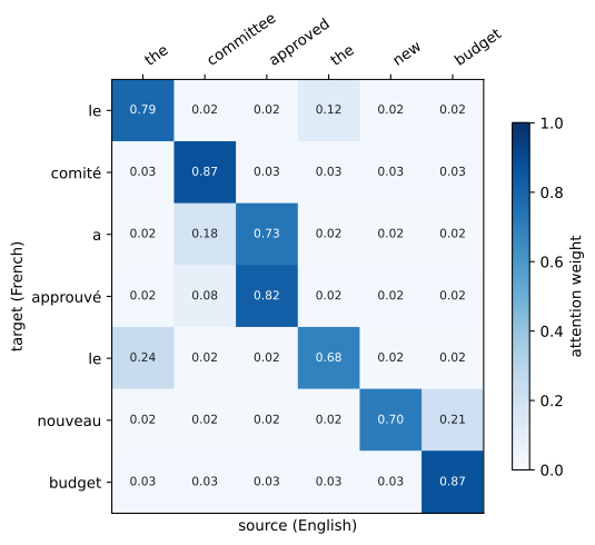
An encoder reads the source sentence and produces a sequence of contextual vectors \(\mathbf{h}_1, \ldots, \mathbf{h}_n\), one per source token. A decoder generates the target sentence one token at a time, each step conditioned on the tokens generated so far and on the source. The original encoder-decoder compressed the whole source into one fixed vector, a bottleneck that made long sentences fail. Attention removes the bottleneck: at each decoding step \(t\), the decoder computes a weighted average of all encoder vectors, with weights reflecting how relevant each source token is to the next target token:

where \(\mathbf{s}_t\) is the decoder state and the score may be a dot product or a small neural network. The context vector \(\mathbf{c}_t\) is combined with the decoder state to predict the next token. Attention weights often resemble word alignments, though they are not guaranteed to be interpretable as such. In the transformer, the same idea appears as cross-attention, in which decoder queries attend to encoder keys and values (Lesson 6).

Training data and techniques

Neural MT systems are trained to maximize the probability of reference translations given sources, using teacher forcing (feeding the correct previous target tokens during training). Their quality depends heavily on data:

• Parallel data come from governments (parliamentary proceedings, legislation), international organizations, translated websites, subtitles and books, filtered for alignment errors and noise. High-resource pairs such as English-French have hundreds of millions of sentence pairs; most of the world's roughly 7,000 languages have almost none.
• Back-translation creates synthetic parallel data from monolingual target-language text: a reverse model translates target sentences into the source language, and the resulting pairs (synthetic source, real target) are added to training. Because the target side is genuine fluent text, back-translation substantially improves quality, especially in low-resource settings.
• Subword vocabularies shared between languages (Lesson 1) handle rare words, names and morphologically rich languages.
• Domain adaptation fine-tunes general models on in-domain data (legal, medical, technical) to learn its terminology and style.
• Terminology constraints and translation memories ensure consistent translation of key terms, essential in professional settings.

Decoding: beam search and length

At inference, the model must find a high-probability target sequence. Greedy decoding picks the most probable token at each step; beam search keeps the \(k\) best partial translations (typically \(k = 4\) to 10) and expands each, keeping a better overall sequence (Lesson 4). Because each additional token multiplies in a probability below one, raw log-probability favours short outputs, which can cut translations short. Length normalization divides the log-probability by a length penalty, such as \(\mathrm{lp}(Y) = ((5 + |Y|)/6)^\alpha\) used in Google's neural MT system:

import math

# Candidate translations with per-token log-probabilities from a model (made-up but typical values)
cands = {
    "the meeting is cancelled": [-0.4, -0.9, -0.3, -1.1],
    "the meeting has been cancelled because of the storm": [-0.4, -0.9, -0.5, -0.2, -0.6, -0.4, -0.2, -0.3, -0.3],
    "meeting cancelled": [-2.2, -1.3],
}
for alpha in (0.0, 0.6, 1.0):
    print(f"length normalization alpha = {alpha}:")
    for text, lps in cands.items():
        total = sum(lps)
        lp = ((5 + len(lps)) / 6) ** alpha                  # length penalty used in Google NMT
        print(f"   score {total / lp:6.2f}  (log-prob {total:5.2f}, {len(lps)} tokens)  {text}")
    best = max(cands, key=lambda t: sum(cands[t]) / ((5 + len(cands[t])) / 6) ** alpha)
    print(f"   chosen: {best}")

length normalization alpha = 0.0:
   score  -2.70  (log-prob -2.70, 4 tokens)  the meeting is cancelled
   score  -3.80  (log-prob -3.80, 9 tokens)  the meeting has been cancelled because of the storm
   score  -3.50  (log-prob -3.50, 2 tokens)  meeting cancelled
   chosen: the meeting is cancelled
length normalization alpha = 0.6:
   score  -2.12  (log-prob -2.70, 4 tokens)  the meeting is cancelled
   score  -2.29  (log-prob -3.80, 9 tokens)  the meeting has been cancelled because of the storm
   score  -3.19  (log-prob -3.50, 2 tokens)  meeting cancelled
   chosen: the meeting is cancelled
length normalization alpha = 1.0:
   score  -1.80  (log-prob -2.70, 4 tokens)  the meeting is cancelled
   score  -1.63  (log-prob -3.80, 9 tokens)  the meeting has been cancelled because of the storm
   score  -3.00  (log-prob -3.50, 2 tokens)  meeting cancelled
   chosen: the meeting has been cancelled because of the storm

Without normalization, the short translation wins even though the longer one is more faithful and has better per-token probabilities. With \(\alpha = 1\), the full translation is chosen. The strength of normalization is tuned on validation data; too much favours long, rambling outputs. Neural MT also exhibits a known paradox: very large beams can produce worse translations, including empty outputs, a symptom of model probabilities that do not perfectly reflect quality.

Evaluating translation

Human evaluation is the gold standard: professional translators rate adequacy (is the meaning preserved?) and fluency, or rank system outputs, or annotate specific errors (the MQM framework classifies errors by type and severity). Because it is slow and expensive, automatic metrics are used during development:

• BLEU (bilingual evaluation understudy) computes the geometric mean of modified n-gram precisions (clipped by counts in the references) for n = 1 to 4, multiplied by a brevity penalty for outputs shorter than the reference: \(\mathrm{BLEU} = \mathrm{BP} \cdot \exp\left(\frac14\sum_{n=1}^{4}\log p_n\right)\). It is computed over a whole test set, not individual sentences, where it is unstable.
• chrF computes an F-score over character n-grams, rewarding partial word matches and handling morphology better than BLEU.
• Learned metrics such as COMET and BLEURT use neural models trained on human judgements to score a translation against the source and reference, correlating much better with human ratings, and are now preferred in research and evaluation campaigns such as the WMT shared tasks.

import math
from collections import Counter

def ngrams(toks, n):
    return Counter(tuple(toks[i:i + n]) for i in range(len(toks) - n + 1))

def bleu(hyp, refs, max_n=4):
    hyp = hyp.split(); refs = [r.split() for r in refs]
    precisions = []
    for n in range(1, max_n + 1):
        h = ngrams(hyp, n)
        max_ref = Counter()
        for r in refs:
            for g, c in ngrams(r, n).items(): max_ref[g] = max(max_ref[g], c)
        clipped = sum(min(c, max_ref[g]) for g, c in h.items())
        precisions.append(max(clipped, 1e-9) / max(sum(h.values()), 1))
    closest = min((abs(len(r) - len(hyp)), len(r)) for r in refs)[1]
    bp = 1.0 if len(hyp) > closest else math.exp(1 - closest / len(hyp))
    return bp * math.exp(sum(math.log(p) for p in precisions) / max_n), precisions, bp

def chrf(hyp, ref, n=6, beta=2):
    scores = []
    for k in range(1, n + 1):
        h = Counter(hyp[i:i + k] for i in range(len(hyp) - k + 1)); r = Counter(ref[i:i + k] for i in range(len(ref) - k + 1))
        m = sum((h & r).values())
        p = m / max(sum(h.values()), 1); rc = m / max(sum(r.values()), 1)
        scores.append(0 if p + rc == 0 else (1 + beta ** 2) * p * rc / (beta ** 2 * p + rc))
    return sum(scores) / n

refs = ["the committee approved the new budget on tuesday", "on tuesday the committee passed the new budget"]
for hyp in ["the committee approved the new budget on tuesday", "the committee passed the budget on tuesday",
            "on tuesday the new budget was approved by the committee", "the committee approved", "budget new the approved committee the tuesday on"]:
    b, p, bp = bleu(hyp, refs)
    print(f"BLEU {b * 100:5.1f}  chrF {chrf(hyp, refs[0]) * 100:5.1f}  BP {bp:.2f}  | {hyp}")

BLEU 100.0  chrF 100.0  BP 1.00  | the committee approved the new budget on tuesday
BLEU  51.5  chrF  71.1  BP 0.87  | the committee passed the budget on tuesday
BLEU   0.2  chrF  82.4  BP 1.00  | on tuesday the new budget was approved by the committee
BLEU   0.1  chrF  48.3  BP 0.19  | the committee approved
BLEU   0.0  chrF  72.8  BP 1.00  | budget new the approved committee the tuesday on

The exact match scores 100 on both. A good paraphrase in passive voice scores almost zero BLEU, because it shares no four-word sequence with either reference, while chrF gives it a high score. A word salad of the right words also scores zero BLEU but a misleadingly high chrF, showing that character overlap ignores order too much. The truncated output is punished by BLEU's brevity penalty. No surface metric captures meaning reliably, which is why learned metrics and human evaluation are used for important decisions, and why sentence-level BLEU (which requires smoothing to avoid zeros) should not be used to judge individual translations.

Multilingual and low-resource translation

A single multilingual model can translate between many languages, sharing parameters across them. Low-resource languages benefit from transfer: what the model learns from high-resource pairs helps it with related languages, and it can even translate between pairs never seen together in training (zero-shot translation). Meta's No Language Left Behind model covered 200 languages, with evaluation benchmarks created for many low-resource languages for the first time.

Challenges remain: quality for low-resource languages lags far behind; scripts, dialects and code-switching complicate tokenization and data; and data for Indigenous languages raise questions of community consent and data sovereignty. In Canada, projects developing language technology for Indigenous languages, such as Inuktitut and Cree, emphasize partnership with language communities, which hold rights over how their languages are used.

Translation in practice

Machine translation is used in three broad modes: gisting (understanding foreign-language content where rough quality suffices), assisting human translators through post-editing (correcting MT output, now the dominant workflow in professional translation), and fully automatic publication where quality is high enough and errors are low-risk. In Canada, federal institutions must communicate in both official languages under the Official Languages Act, and the federal Translation Bureau combines professional translators with machine translation tools, with human review for published material. Quebec's Charter of the French Language sets requirements for the use of French in commerce and employment that affect how organizations use MT. Risky domains, such as health, legal and safety information, require human review because a fluent but wrong translation can cause harm.