Sequence models

Language is sequential: the meaning of a word depends on what came before it, sometimes many words before. "The keys to the cabinet in the hallway are missing" requires matching "are" with "keys", seven words back, not with "hallway". Bag-of-words models ignore order, and n-gram models see only a few words of context. This lesson covers neural models designed for sequences: recurrent neural networks (RNNs), their gated variants LSTM and GRU, bidirectional and encoder-decoder architectures, and the decoding algorithms used to generate text. RNNs dominated NLP from about 2014 to 2018; transformers (Lesson 6) have since replaced them for most tasks, but the problems RNNs faced explain why transformers were designed as they were, and recurrent ideas are returning in efficient modern architectures.

Sequence tasks

NLP tasks on sequences fall into a few patterns:

• Sequence classification: one label for a whole input, such as sentiment, topic or spam detection.
• Sequence labelling (tagging): one label per token, such as part-of-speech tagging or named entity recognition (NER). NER often uses the BIO scheme: B-PER marks the beginning of a person's name, I-PER a token inside it, and O a token outside any entity, so "Ada Lovelace visited London" is tagged B-PER I-PER O B-LOC.
• Sequence-to-sequence (seq2seq): an output sequence of different length from the input, such as translation, summarization and speech recognition.
• Language modelling and generation: predicting the next token repeatedly to produce text.

Neural language models

In 2003, Bengio and colleagues proposed a neural language model that replaced n-gram counts with a neural network: the embeddings of the previous \(n-1\) words are concatenated and passed through a hidden layer and a softmax output over the vocabulary. Because similar words have similar embeddings, the model generalizes from "the cat sat" to "the kitten sat", which n-gram models cannot. Its context is still fixed, though: a 5-word window cannot see the subject of a long sentence.

Recurrent neural networks

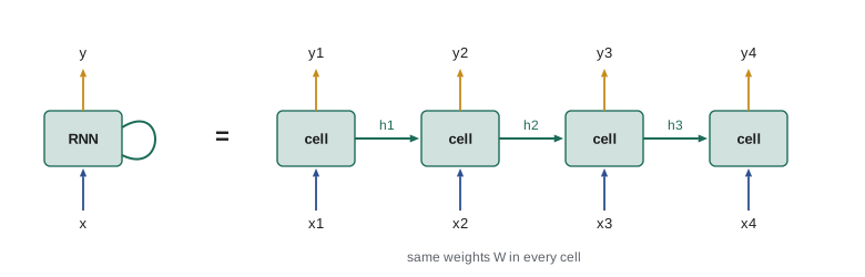
A recurrent neural network processes a sequence one element at a time, maintaining a hidden state \(\mathbf{h}_t\) that summarizes everything seen so far. At each step it combines the previous hidden state with the current input:

The same weights are used at every time step, so an RNN can process sequences of any length with a fixed number of parameters, and what it learns about a pattern at one position applies at every position. As a language model, the RNN reads one token per step and predicts the next from \(\mathbf{h}_t\), which in principle depends on the entire history.

Training and vanishing gradients

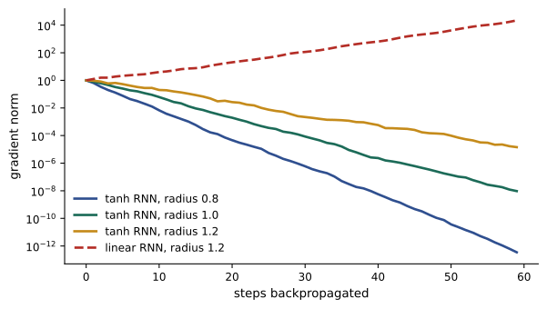
RNNs are trained by backpropagation through time (BPTT): the network is unrolled over the sequence, the loss is summed over all steps, and gradients flow backwards through every step. The gradient reaching step \(t-k\) from step \(t\) is a product of \(k\) Jacobian matrices:

If the factors shrink vectors, the product shrinks exponentially and the gradient vanishes, so the network cannot learn long-range dependencies. If they grow vectors, the gradient explodes and training becomes unstable. The spectral radius of \(W_{hh}\) (its largest eigenvalue magnitude) largely decides which, and the tanh derivative, at most 1 and much smaller when units saturate, pushes towards vanishing.

import numpy as np

rng = np.random.default_rng(0)
d, T = 64, 60
for rho in (0.8, 1.0, 1.2):
    W = rng.normal(0, 1, (d, d))
    W *= rho / max(abs(np.linalg.eigvals(W)))       # set the spectral radius
    h = np.zeros(d)
    hs = []
    x = rng.normal(0, 1, (T, d)) * 0.5
    for t in range(T):                              # forward pass of a tanh RNN
        h = np.tanh(W @ h + x[t])
        hs.append(h)
    g = np.ones(d) / np.sqrt(d)                     # gradient arriving at the last state
    norms = {}
    for k, t in enumerate(range(T - 1, -1, -1)):    # backpropagate through time
        norms[k] = np.linalg.norm(g)
        g = W.T @ (g * (1 - hs[t] ** 2))
    print(f"spectral radius {rho}: |grad| after 1, 10, 30, 59 steps back:",
          " ".join(f"{norms[k]:.1e}" for k in (1, 10, 30, 59)))
    # the same with a linear RNN (no tanh) shows pure exponential growth or decay
    g = np.ones(d) / np.sqrt(d)
    for _ in range(59):
        g = W.T @ g
    print(f"   linear RNN after 59 steps: {np.linalg.norm(g):.1e}")

spectral radius 0.8: |grad| after 1, 10, 30, 59 steps back: 6.5e-01 6.7e-03 5.9e-07 3.5e-13
   linear RNN after 59 steps: 9.7e-07
spectral radius 1.0: |grad| after 1, 10, 30, 59 steps back: 7.8e-01 6.1e-02 8.5e-05 9.5e-09
   linear RNN after 59 steps: 2.2e-01
spectral radius 1.2: |grad| after 1, 10, 30, 59 steps back: 9.4e-01 2.0e-01 2.2e-03 1.4e-05
   linear RNN after 59 steps: 2.2e+04

With spectral radius 0.8, the gradient falls by about 12 orders of magnitude over 59 steps. Even at 1.0 and 1.2, the saturating tanh makes gradients vanish in the nonlinear network, while the linear network with radius 1.2 explodes to 22,000. In practice, exploding gradients are handled by gradient clipping (rescaling the gradient when its norm exceeds a threshold, AI-310), while vanishing gradients required a change of architecture.

LSTM and GRU

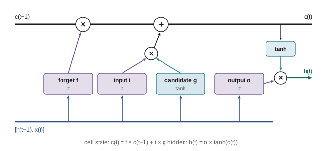
The long short-term memory (LSTM) network, introduced by Hochreiter and Schmidhuber in 1997, adds a cell state \(\mathbf{c}_t\) that is updated additively and controlled by gates, vectors of values between 0 and 1 computed by sigmoid functions:

The forget gate \(\mathbf{f}_t\) decides how much of the old cell state to keep, the input gate \(\mathbf{i}_t\) how much new information \(\mathbf{g}_t\) to write, and the output gate \(\mathbf{o}_t\) how much of the cell to expose as the hidden state. When the forget gate is near 1 and the input gate near 0, the cell state passes through unchanged, and so does its gradient: the additive path acts as a "gradient highway" across many steps. Initializing the forget-gate bias to a positive value (such as 1 or 2) helps networks remember by default.

import numpy as np

sig = lambda z: 1 / (1 + np.exp(-z))
T = 100
x = np.zeros(T); x[0] = 1.0                         # a single signal at the first step, then silence

def simple_rnn(w):
    h = 0.0
    for t in range(T):
        h = np.tanh(w * h + 2.0 * x[t])
    return h

def lstm(forget_bias):
    c = h = 0.0
    for t in range(T):
        f = sig(forget_bias)                        # forget gate (input-independent here)
        i = sig(-4 + 8 * x[t])                      # input gate opens only when x = 1
        g = np.tanh(2.0 * x[t])                     # candidate value
        c = f * c + i * g                           # additive cell-state update
        o = sig(4.0)
        h = o * np.tanh(c)
    return c, h

print("simple RNN, w = 0.9: memory after 100 steps =", f"{simple_rnn(0.9):.2e}")
print("simple RNN, w = 1.5: memory after 100 steps =", f"{simple_rnn(1.5):.3f}  (saturated, cannot forget)")
for b in (2, 5, 10):
    c, h = lstm(b)
    print(f"LSTM forget bias {b:2d}: f = {sig(b):.5f}, cell after 100 steps = {c:.3f}")

simple RNN, w = 0.9: memory after 100 steps = 1.48e-05
simple RNN, w = 1.5: memory after 100 steps = 0.859  (saturated, cannot forget)
LSTM forget bias  2: f = 0.88080, cell after 100 steps = 0.000
LSTM forget bias  5: f = 0.99331, cell after 100 steps = 0.487
LSTM forget bias 10: f = 0.99995, cell after 100 steps = 0.942

The simple RNN either forgets the signal almost completely (\(w = 0.9\)) or saturates and holds a value permanently, unable to forget anything (\(w = 1.5\)). The LSTM's memory is controlled by its forget gate: with \(f = 0.88\) the stored value vanishes, with \(f = 0.993\) half remains after 100 steps (\(0.993^{100} = 0.51\)), and with \(f = 0.99995\) almost all of it does. In a trained LSTM, the gates are computed from the input, so the network learns when to keep, overwrite and output information.

The gated recurrent unit (GRU, 2014) simplifies the LSTM to two gates (update and reset) and no separate cell state, with fewer parameters and similar performance on many tasks.

Bidirectional and stacked RNNs

For tagging and classification, the whole input is available at once, so a token's label can depend on words after it as well as before ("Washington" is a person in "Washington said" and a place in "Washington state"). A bidirectional RNN runs one RNN forwards and another backwards and concatenates their hidden states at each position. Stacking several RNN layers, each taking the previous layer's hidden states as input, increases capacity. Bidirectional LSTMs with a conditional random field (CRF) output layer, which scores whole tag sequences so that invalid transitions such as O followed by I-PER are discouraged, were the standard NER architecture before transformers. ELMo (2018) used the hidden states of a deep bidirectional LSTM language model as contextual word embeddings (Lesson 2).

Encoder-decoder models

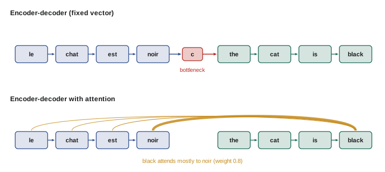
For seq2seq tasks such as translation, an encoder RNN reads the source sentence into its final hidden state, and a decoder RNN, initialized with that state, generates the target sentence one token at a time, each step conditioned on the previously generated token. During training, the decoder is fed the correct previous token rather than its own prediction, a technique called teacher forcing. This speeds training but creates exposure bias: at inference time the model must continue from its own, possibly wrong, outputs, a situation it never saw in training.

The basic encoder-decoder has a bottleneck: the entire source sentence must be compressed into one fixed-size vector, and translation quality fell sharply for long sentences. In 2014, Bahdanau, Cho and Bengio added attention: at each decoding step, the decoder computes a weighted average of all encoder hidden states, with weights based on how relevant each source position is to the current output. The decoder can then look back at the relevant source words directly. Attention dramatically improved translation and, as Lesson 6 shows, turned out to be powerful enough to replace recurrence entirely.

Decoding: generating text

A trained language model gives a probability distribution over the next token. Turning this into text requires a decoding strategy:

• Greedy decoding picks the most probable token at each step. It is fast but can miss sequences whose first token is less likely but whose total probability is higher.
• Beam search keeps the \(k\) most probable partial sequences (the beam) at each step, extends each by every possible token, and keeps the top \(k\) again. It finds higher-probability outputs and is standard for translation and speech recognition, usually with a length penalty because shorter sequences have higher probabilities.
• Sampling draws the next token from the distribution, producing varied text; it is used for open-ended generation, where the most probable text tends to be bland and repetitive.

import math

# a toy next-word model: probabilities depend only on the previous word
P = {"<s>":  {"the": 0.5, "a": 0.4, "</s>": 0.1},
     "the":  {"dog": 0.4, "cat": 0.35, "</s>": 0.25},
     "a":    {"small": 0.9, "</s>": 0.1},
     "small": {"cat": 0.9, "</s>": 0.1},
     "dog":  {"barked": 0.3, "</s>": 0.7},
     "cat":  {"</s>": 0.9, "sat": 0.1},
     "barked": {"</s>": 1.0}, "sat": {"</s>": 1.0}}

def greedy():
    seq, lp = ["<s>"], 0.0
    while seq[-1] != "</s>":
        w, p = max(P[seq[-1]].items(), key=lambda kv: kv[1])
        seq.append(w); lp += math.log(p)
    return seq[1:], lp

def beam(width, max_len=6):
    beams = [(["<s>"], 0.0)]
    done = []
    for _ in range(max_len):
        cand = []
        for seq, lp in beams:
            for w, p in P[seq[-1]].items():
                cand.append((seq + [w], lp + math.log(p)))
        cand.sort(key=lambda c: -c[1])
        beams = []
        for seq, lp in cand[:width]:
            (done if seq[-1] == "</s>" else beams).append((seq, lp))
        if not beams:
            break
    seq, lp = max(done, key=lambda c: c[1])
    return seq[1:], lp

s, lp = greedy()
print("greedy:      ", " ".join(s), f" p = {math.exp(lp):.3f}")
for k in (1, 2, 3):
    s, lp = beam(k)
    print(f"beam width {k}:", " ".join(s), f" p = {math.exp(lp):.3f}")

greedy:       the dog </s>  p = 0.140
beam width 1: the dog </s>  p = 0.140
beam width 2: a small cat </s>  p = 0.292
beam width 3: a small cat </s>  p = 0.292

Greedy decoding chooses "the" (0.5) over "a" (0.4) and ends with "the dog", probability 0.14. Beam search with width 2 keeps "a" alive and finds "a small cat", with probability 0.29, more than twice as likely. Beam width 1 is identical to greedy.

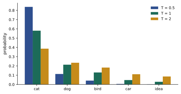
Sampling is controlled by several parameters. Temperature \(T\) divides the logits (the scores before softmax) before sampling:

Low temperature sharpens the distribution towards greedy decoding; high temperature flattens it, increasing diversity and the risk of nonsense. Top-k sampling keeps only the \(k\) most probable tokens; nucleus (top-p) sampling keeps the smallest set of tokens whose cumulative probability exceeds \(p\) (such as 0.9), adapting the number of candidates to how confident the model is.

Limits of recurrence

RNNs process tokens one after another, so computation cannot be parallelized across a sequence during training: step 100 must wait for step 99. This makes training on long sequences and huge corpora slow on GPUs, which excel at parallel work. Even LSTMs struggle to use information hundreds of tokens back, and information must pass through every intermediate step. The transformer, introduced in 2017, removed recurrence and connected every position directly to every other with attention, solving both problems at the cost of computation that grows with the square of the sequence length. Since 2023, state space models such as Mamba and linear-attention architectures have revived recurrent ideas, offering constant memory per generated token, and some production models combine them with attention layers.

Lesson 5 applies encoder-decoder models and beam search to machine translation, and Lesson 6 shows how attention replaced recurrence.