Joint distributions, covariance and correlation

Interesting questions usually involve more than one random quantity: the claim frequency and the claim size, the height and weight of a patient, the temperature and the electricity demand, the returns of two stocks. To answer them we need the joint distribution, which describes how the variables behave together, not just one at a time. This lesson defines joint pmfs and densities, recovers the individual (marginal) distributions from them, defines conditional distributions and independence for random variables, and introduces covariance and correlation, the standard measures of how two variables move together. It ends with the variance of a sum of dependent variables, which is the key to portfolio risk and to the finite population correction of lesson 7.

Joint pmfs

For discrete \(X\) and \(Y\), the joint pmf is \(p(x, y) = P(X = x, Y = y)\). It is non-negative and sums to 1 over all pairs, and \(P((X, Y) \in B) = \sum_{(x,y) \in B} p(x, y)\). The marginal pmfs come from summing out the other variable: \(p_X(x) = \sum_y p(x, y)\) and \(p_Y(y) = \sum_x p(x, y)\), which is the law of total probability. Joint pmfs of two variables are conveniently written as tables, with the marginals in the margins, which is where the name comes from.

Here is an example from a car insurer. Let \(X\) be the number of claims a policy has in a year (0, 1 or 2) and \(Y\) whether the driver is under 25 (1 if so). Suppose the joint pmf is \(p(0,0) = 0.56\), \(p(1,0) = 0.12\), \(p(2,0) = 0.02\), \(p(0,1) = 0.18\), \(p(1,1) = 0.08\), \(p(2,1) = 0.04\). Then \(P(Y = 1) = 0.30\), \(P(X = 0) = 0.74\), \(P(X = 1) = 0.20\), \(P(X = 2) = 0.06\). The marginals alone cannot tell us whether young drivers claim more; the joint table can.

Joint densities

Continuous \(X\) and \(Y\) have a joint density \(f(x, y) \ge 0\) if \(P((X, Y) \in B) = \iint_B f(x, y)\,dx\,dy\) for regions \(B\) in the plane. The density integrates to 1 over the plane. Marginal densities integrate out the other variable: \(f_X(x) = \int f(x, y)\,dy\). Probabilities are volumes under the density surface, and the practical skill is setting up the limits of integration for the region \(B\), which usually means drawing it.

Conditional distributions

The conditional pmf of \(Y\) given \(X = x\) is \(p_{Y \mid X}(y \mid x) = p(x, y)/p_X(x)\), defined when \(p_X(x) > 0\). For continuous variables the conditional density is \(f_{Y \mid X}(y \mid x) = f(x, y)/f_X(x)\). Strictly, conditioning on an event of probability zero needs care, but the formula is the limit of conditioning on \(x \le X \le x + h\) as \(h \to 0\), and it behaves as expected. In the insurance example, \(P(X \ge 1 \mid Y = 1) = 0.12/0.30 = 0.40\) while \(P(X \ge 1 \mid Y = 0) = 0.14/0.70 = 0.20\): young drivers are twice as likely to claim.

The conditional expectation \(E[Y \mid X = x] = \sum_y y\,p_{Y \mid X}(y \mid x)\), or the corresponding integral, is the mean of the conditional distribution. As a function of \(x\) it is called the regression function of \(Y\) on \(X\). Writing \(E[Y \mid X]\) for this function evaluated at the random \(X\) gives a random variable, and the law of total expectation says \(E[E[Y \mid X]] = E[Y]\): average the conditional means, weighting by the distribution of \(X\). A companion result, the law of total variance, \(\operatorname{Var}(Y) = E[\operatorname{Var}(Y \mid X)] + \operatorname{Var}(E[Y \mid X])\), splits the total variance into the part within groups and the part between them. Actuaries use it to separate the randomness of claims for a known risk from the uncertainty about which risk a policy is.

Independence

Random variables \(X\) and \(Y\) are independent if the joint distribution factors into the marginals: \(p(x, y) = p_X(x)p_Y(y)\) for all \(x, y\) in the discrete case, or \(f(x, y) = f_X(x)f_Y(y)\) in the continuous case. Equivalently, every conditional distribution of \(Y\) given \(X = x\) equals the marginal of \(Y\). A useful test: if the joint density factors as \(g(x)h(y)\) on a product region (a rectangle, possibly infinite), the variables are independent. The triangle example fails the test even though its density is constant, because the region is not a rectangle: knowing \(X = 0.1\) forces \(Y < 0.1\).

Covariance

The covariance of \(X\) and \(Y\) is

It is positive when large values of \(X\) tend to go with large values of \(Y\), negative when large values of one go with small values of the other, and zero when neither tendency dominates. Covariance is bilinear: \(\operatorname{Cov}(aX + bY, Z) = a\operatorname{Cov}(X, Z) + b\operatorname{Cov}(Y, Z)\), and it is symmetric, with \(\operatorname{Cov}(X, X) = \operatorname{Var}(X)\). If \(X\) and \(Y\) are independent their covariance is zero, because \(E[XY] = E[X]E[Y]\). The converse is false. If \(X\) is uniform on \(\{-1, 0, 1\}\) and \(Y = X^2\), then \(E[XY] = E[X^3] = 0 = E[X]E[Y]\), so the covariance is zero, but \(Y\) is a function of \(X\). Covariance only detects linear association.

Variance of a sum

Expanding the square in \(\operatorname{Var}(X + Y) = E[(X - \mu_X + Y - \mu_Y)^2]\) gives

Dependence enters only through covariances. Positive covariances inflate the variance of a total and negative ones shrink it. This single formula explains diversification. An insurer with \(n\) policies, each with loss variance \(\sigma^2\) and pairwise covariance \(\rho\sigma^2\), has total loss variance \(n\sigma^2 + n(n-1)\rho\sigma^2\). Per policy, the variance is \(\sigma^2/n + (1 - 1/n)\rho\sigma^2\), which falls to \(\rho\sigma^2\), not to zero, as \(n\) grows. Independent risks diversify away; correlated risks, such as homes in the same flood plain, do not.

The same formula gives the hypergeometric variance. With indicators \(I_j\) for successes on draw \(j\), \(\operatorname{Var}(I_j) = p(1 - p)\) with \(p = K/N\), and for \(i \ne j\), \(E[I_iI_j] = \frac{K}{N}\cdot\frac{K - 1}{N - 1}\), so \(\operatorname{Cov}(I_i, I_j) = -\frac{p(1-p)}{N-1}\). Adding \(n\) variances and \(n(n-1)\) covariances gives \(np(1 - p)\Big(1 - \frac{n - 1}{N - 1}\Big) = np(1-p)\frac{N - n}{N - 1}\), the finite population correction.

Correlation

Covariance depends on units: measure \(X\) in centimeters instead of meters and the covariance grows by a factor of 100. The correlation coefficient removes the units:

Correlation always lies in \([-1, 1]\). Proof: for any \(t\), \(0 \le \operatorname{Var}(Y - tX) = \sigma_Y^2 - 2t\operatorname{Cov}(X, Y) + t^2\sigma_X^2\). A quadratic in \(t\) that is never negative has discriminant at most zero, so \(\operatorname{Cov}(X, Y)^2 \le \sigma_X^2\sigma_Y^2\). This is the Cauchy–Schwarz inequality for random variables. Equality \(|\rho| = 1\) holds exactly when \(\operatorname{Var}(Y - tX) = 0\) for some \(t\), that is when \(Y\) is a linear function of \(X\) with probability 1. Correlation measures the strength of the linear relationship. A correlation near zero does not mean no relationship, as the \(Y = X^2\) example shows, and a strong correlation does not mean causation: ice cream sales and drownings are correlated because both rise in hot weather.

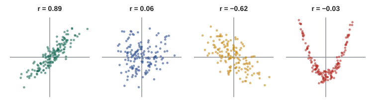
The bivariate normal

The most important joint density is the bivariate normal. With standard normal marginals and correlation \(\rho\), its density is \(f(x, y) = \frac{1}{2\pi\sqrt{1 - \rho^2}}e^{-Q/2}\), where \(Q = (x^2 - 2\rho xy + y^2)/(1 - \rho^2)\). Its contours are ellipses. It can be built from two independent standard normals \(Z_1, Z_2\) by setting \(X = Z_1\) and \(Y = \rho Z_1 + \sqrt{1 - \rho^2}Z_2\). Two facts make it special. Its conditional distributions are normal, with \(E[Y \mid X = x] = \rho x\) and \(\operatorname{Var}(Y \mid X = x) = 1 - \rho^2\), so the regression is a straight line. And for bivariate normal variables, zero correlation does imply independence, because \(\rho = 0\) makes the density factor. This is the setting in which correlation tells the whole story about dependence.

import random, math
from statistics import mean

# insurance table: rows X = 0, 1, 2 claims; columns Y = 0 (25+), 1 (under 25)
p = {(0, 0): .56, (1, 0): .12, (2, 0): .02, (0, 1): .18, (1, 1): .08, (2, 1): .04}
EX = sum(x * q for (x, y), q in p.items()); EY = sum(y * q for (x, y), q in p.items())
EXY = sum(x * y * q for (x, y), q in p.items())
VX = sum(x * x * q for (x, y), q in p.items()) - EX ** 2; VY = EY - EY ** 2
cov = EXY - EX * EY
print(f"E[X] = {EX:.2f}, E[Y] = {EY:.2f}, Cov = {cov:.4f}, corr = {cov / math.sqrt(VX * VY):.4f}")
for y in (0, 1):
    py = sum(q for (x, yy), q in p.items() if yy == y)
    print(f"E[X | Y = {y}] = {sum(x * q for (x, yy), q in p.items() if yy == y) / py:.3f}")

# zero covariance without independence
xs = [-1, 0, 1]
print("Cov(X, X^2) for X uniform on {-1,0,1}:", mean([x ** 3 for x in xs]) - mean(xs) * mean([x * x for x in xs]))

# bivariate normal by construction, rho = 0.7
rng = random.Random(251); rho = 0.7
pairs = []
for _ in range(100_000):
    z1, z2 = rng.gauss(0, 1), rng.gauss(0, 1)
    pairs.append((z1, rho * z1 + math.sqrt(1 - rho ** 2) * z2))
mx = mean(a for a, b in pairs); my = mean(b for a, b in pairs)
sxy = mean((a - mx) * (b - my) for a, b in pairs)
sx = math.sqrt(mean((a - mx) ** 2 for a, b in pairs)); sy = math.sqrt(mean((b - my) ** 2 for a, b in pairs))
near1 = [b for a, b in pairs if 0.95 < a < 1.05]
print(f"sample correlation {sxy / (sx * sy):.3f};  E[Y | X ~ 1] = {mean(near1):.3f} (0.7)")

# diversification: per-policy variance with pairwise correlation 0.05
for n in (1, 10, 100, 10_000):
    print(f"n = {n:>6}: variance per policy {1 / n + (1 - 1 / n) * 0.05:.4f}")

E[X] = 0.32, E[Y] = 0.30, Cov = 0.0640, corr = 0.2404
E[X | Y = 0] = 0.229
E[X | Y = 1] = 0.533
Cov(X, X^2) for X uniform on {-1,0,1}: 0.0
sample correlation 0.701;  E[Y | X ~ 1] = 0.713 (0.7)
n =      1: variance per policy 1.0000
n =     10: variance per policy 0.1450
n =    100: variance per policy 0.0595
n =  10000: variance per policy 0.0501

The multinomial distribution

The binomial generalizes to experiments with more than two outcomes. In \(n\) independent trials, each giving outcome \(i\) with probability \(p_i\) for \(i = 1, \dots, r\), the counts \((N_1, \dots, N_r)\) have the multinomial distribution: \(P(N_1 = n_1, \dots, N_r = n_r) = \frac{n!}{n_1!\cdots n_r!}p_1^{n_1}\cdots p_r^{n_r}\) when the \(n_i\) sum to \(n\). Each count on its own is binomial, \(N_i \sim \text{Bin}(n, p_i)\). The counts are dependent, because they must add up to \(n\): a large count in one category leaves less room for the others. Writing each count as a sum of indicators and using bilinearity gives \(\operatorname{Cov}(N_i, N_j) = -np_ip_j\) for \(i \ne j\), so the correlation is negative. In an election poll of 1,000 voters choosing among three parties with support 40%, 35% and 25%, the counts for the first two parties have covariance \(-1000(0.4)(0.35) = -140\), and the variance of the difference in their counts, the quantity that decides who is ahead, is \(240 + 227.5 + 2(140) = 747.5\), larger than the sum of the two variances.