Discrete random variables

So far we have assigned probabilities to events. Most questions, though, are about numbers: how many claims, how many defective parts, how many patients respond, how long until the first failure. A random variable is a rule that attaches a number to each outcome of an experiment, and its distribution records how probability is spread over the possible values. This lesson defines random variables in general and develops the discrete case, where the values can be listed. Lesson 5 does the continuous case, lesson 6 defines expectation, and lessons 7 and 8 catalog the distributions you will use most.

Random variables

A random variable is a function \(X : \Omega \to \mathbb{R}\). The function itself is not random; what is random is the outcome \(\omega\) at which it is evaluated. Toss a coin three times and let \(X\) be the number of heads. Then \(X(HHT) = 2\), \(X(TTT) = 0\), and so on. Several random variables can be defined on the same experiment: \(Y\) might be the number of the toss on which the first head appears, and \(Z\) the length of the longest run. Each answers a different question about the same outcome.

Events defined by random variables are written in shorthand. \(\{X = 2\}\) means the set of outcomes \(\{\omega : X(\omega) = 2\} = \{HHT, HTH, THH\}\), and \(\{X \le 1\}\) means \(\{\omega : X(\omega) \le 1\}\). So \(P(X = 2) = 3/8\) for fair tosses. Formally a random variable must be such that every set \(\{X \le x\}\) is an event that has a probability; on the sample spaces of this course that is always true.

The probability mass function

A random variable is discrete if it takes finitely or countably many values \(x_1, x_2, \ldots\). Its probability mass function, or pmf, is \(p(x) = P(X = x)\). Every pmf satisfies two conditions: \(p(x) \ge 0\) for all \(x\), and \(\sum_i p(x_i) = 1\). Conversely, any function with these two properties is the pmf of some random variable. The probability that \(X\) lands in a set \(B\) is obtained by adding: \(P(X \in B) = \sum_{x_i \in B} p(x_i)\), which is just countable additivity.

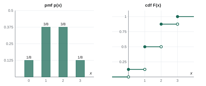
For the number of heads in three fair tosses, \(p(0) = 1/8\), \(p(1) = 3/8\), \(p(2) = 3/8\), \(p(3) = 1/8\). For the toss \(Y\) on which the first head appears in an unlimited sequence, \(p(k) = (1/2)^k\) for \(k = 1, 2, \ldots\), because the first \(k - 1\) tosses must be tails and the \(k\)th a head. These add to 1 by the geometric series. Both are examples of distributions we name in lesson 7: the binomial and the geometric.

The cumulative distribution function

Every random variable, discrete or not, has a cumulative distribution function, or cdf, \(F(x) = P(X \le x)\) for all real \(x\). For a discrete variable \(F\) is a step function that jumps by \(p(x_i)\) at each value \(x_i\) and is flat in between. For three tosses, \(F(x) = 0\) for \(x < 0\), \(1/8\) for \(0 \le x < 1\), \(1/2\) for \(1 \le x < 2\), \(7/8\) for \(2 \le x < 3\), and 1 for \(x \ge 3\).

Every cdf has three properties, and any function with them is the cdf of some random variable:

• \(F\) is non-decreasing: if \(a < b\) then \(F(a) \le F(b)\), because \(\{X \le a\} \subseteq \{X \le b\}\).

• \(F(x) \to 0\) as \(x \to -\infty\) and \(F(x) \to 1\) as \(x \to \infty\).

• \(F\) is right-continuous: \(F(x + h) \to F(x)\) as \(h\) decreases to 0.

The last two follow from continuity of probability (lesson 1). For right-continuity, the events \(\{X \le x + 1/n\}\) decrease to \(\{X \le x\}\), so their probabilities decrease to \(F(x)\). Approaching from the left is different: \(\{X \le x - 1/n\}\) increases to \(\{X < x\}\), so \(F(x^-) = P(X < x)\) and the size of the jump at \(x\) is \(F(x) - F(x^-) = P(X = x)\). The cdf determines the distribution completely: \(P(a < X \le b) = F(b) - F(a)\) for any \(a < b\), and every other probability about \(X\) can be built from these.

Functions of a random variable

If \(X\) is a random variable and \(g\) a function, then \(Y = g(X)\) is another random variable. Its pmf is found by collecting the values of \(X\) that \(g\) sends to the same place: \(p_Y(y) = \sum_{x : g(x) = y} p_X(x)\). If \(X\) is uniform on \(\{-2, -1, 0, 1, 2\}\), then \(Y = X^2\) takes values 0, 1 and 4 with probabilities 1/5, 2/5 and 2/5. Lesson 10 treats the continuous version, where the collecting is done with derivatives.

Indicator variables

The simplest random variable is the indicator of an event \(A\): \(I_A(\omega) = 1\) if \(\omega \in A\) and 0 otherwise. Indicators turn statements about events into arithmetic. \(I_{A \cap B} = I_A I_B\), \(I_{A^c} = 1 - I_A\), and \(I_{A \cup B} = I_A + I_B - I_A I_B\), which is inclusion–exclusion in disguise. Counting random variables are sums of indicators: the number of heads in \(n\) tosses is \(I_{A_1} + \cdots + I_{A_n}\), where \(A_i\) is 'toss \(i\) is heads'. In lesson 6 this decomposition makes expected values almost trivial to compute, even for counts whose distributions are hard to find.

A worked model: insurance claims

Independence of random variables

Discrete random variables \(X\) and \(Y\) are independent if \(P(X = x, Y = y) = P(X = x)P(Y = y)\) for all values \(x\) and \(y\). Equivalently, every event defined by \(X\) is independent of every event defined by \(Y\). For several variables the product must hold for all values simultaneously. Independence is the property that makes sums tractable: if \(X\) and \(Y\) are independent and integer valued, the pmf of \(S = X + Y\) is the convolution

obtained by splitting \(\{S = s\}\) according to the value of \(X\). The pmf of the total of two dice, with its triangular shape rising from 1/36 at 2 to 6/36 at 7 and falling back, is the convolution of two uniform pmfs on \(\{1, \ldots, 6\}\). Convolving again gives three dice and the 25 and 27 of Galileo's problem.

from fractions import Fraction
from collections import Counter
import random

die = {k: Fraction(1, 6) for k in range(1, 7)}

def convolve(p, q):
    out = Counter()
    for a, pa in p.items():
        for b, pb in q.items():
            out[a + b] += pa * pb
    return dict(sorted(out.items()))

two = convolve(die, die)
three = convolve(two, die)
print("two dice:", {s: str(p) for s, p in two.items()})
print("three dice, P(9) =", three[9], " P(10) =", three[10])

# cdf of three dice and a quantile
cum, F = Fraction(0), {}
for s, p in three.items():
    cum += p
    F[s] = cum
median = min(s for s, c in F.items() if c >= Fraction(1, 2))
print("F(10) =", F[10], " median =", median)

# empirical pmf from 60,000 throws of two dice
rng = random.Random(251)
emp = Counter(rng.randint(1, 6) + rng.randint(1, 6) for _ in range(60_000))
worst = max(abs(emp[s] / 60_000 - float(two[s])) for s in two)
print(f"largest gap between simulated and exact pmf: {worst:.4f}")

two dice: {2: '1/36', 3: '1/18', 4: '1/12', 5: '1/9', 6: '5/36', 7: '1/6', 8: '5/36', 9: '1/9', 10: '1/12', 11: '1/18', 12: '1/36'}
three dice, P(9) = 25/216  P(10) = 1/8
F(10) = 1/2  median = 10
largest gap between simulated and exact pmf: 0.0031

Quantiles

The cdf answers 'what is the probability that \(X \le x\)?'. The reverse question, 'below what value does \(X\) fall with probability \(q\)?', is answered by the quantile function \(F^{-1}(q) = \min\{x : F(x) \ge q\}\). The median is \(F^{-1}(1/2)\), and the quartiles are \(F^{-1}(1/4)\) and \(F^{-1}(3/4)\). For a discrete variable the minimum is needed because \(F\) jumps: for three dice \(F(10) = 1/2\) exactly, so the median is 10. Insurers and regulators work with quantiles all the time. The Value at Risk of a portfolio at level 99.5%, the basis of many solvency rules, is the 0.995 quantile of the loss distribution.

The quantile function also gives a recipe for simulation. If \(U\) is uniform on \((0, 1)\), then \(X = F^{-1}(U)\) has cdf \(F\), because \(F^{-1}(U) \le x\) exactly when \(U \le F(x)\). To simulate claim counts with the geometric pmf above, draw \(U\) and return the smallest \(k\) with \(F(k) \ge U\). This inverse transform method, which works for any distribution, is how most random number generators turn uniform numbers into numbers with a prescribed distribution. Lesson 10 proves it carefully for continuous variables.

Mixtures

Real populations are often mixtures. If 20% of drivers are high risk with claim pmf \(p_H\) and 80% low risk with \(p_L\), the claim count of a randomly chosen driver has pmf \(p(k) = 0.2\,p_H(k) + 0.8\,p_L(k)\), by the law of total probability. A mixture of two simple distributions can have a shape neither has, such as two peaks, and fitting mixtures is a large part of applied statistics. Mixtures also show that the pmf of a randomly chosen individual need not describe any individual: no driver has the mixture pmf.

Worked example: a pmf from a game

This example shows a pattern that recurs throughout the course: for maxima, the cdf is simpler than the pmf, because the event \(\{M \le m\}\) is an intersection of independent events. The same idea gives the distribution of the largest of \(n\) independent observations, which underlies the design of dams, sea walls and power grids, where engineers care about the largest flood or the highest demand over many years. For minima, the survival function \(P(\min > m)\) plays the same role.

The example also illustrates how to check a pmf: every value must be non-negative and the values must sum to 1. When a pmf is derived by a long calculation, these two checks catch most algebra errors. A third check is a quick simulation, which costs a few lines of code and confirms that the probabilities match long-run frequencies.

The cdf determines the distribution

Every cdf has three properties: it is non-decreasing, it is right-continuous, and it tends to 0 at \(-\infty\) and to 1 at \(+\infty\). Conversely, any function with these three properties is the cdf of some random variable; the inverse transform method of lesson 5 constructs one. The cdf also determines every probability about \(X\): \(P(a < X \le b) = F(b) - F(a)\), \(P(X < b) = F(b^-)\), the limit from the left, and \(P(X = b) = F(b) - F(b^-)\), the size of the jump at \(b\). This is why the cdf, rather than the pmf or the density, is the object used to define the distribution of any random variable, discrete, continuous or a mixture of both.