Common continuous distributions

Lesson 5 introduced the uniform and exponential densities. This lesson completes the family of continuous distributions used throughout probability and statistics: the gamma, which generalizes the exponential to waiting for several events; the normal, which describes sums of many small effects and is the subject of the central limit theorem in lesson 11; the beta, which lives on \([0, 1]\) and models proportions; and the Weibull and lognormal, workhorses of reliability and of insurance losses. For each we give the density, the story behind it, its mean and variance, and the facts that connect it with the others. STAT-252 adds the chi-square, \(t\) and \(F\) distributions, which are built from these.

The gamma function and the gamma distribution

The gamma function, \(\Gamma(\alpha) = \int_0^\infty x^{\alpha - 1}e^{-x}\,dx\) for \(\alpha > 0\), extends the factorial to real arguments. Integration by parts gives \(\Gamma(\alpha + 1) = \alpha\Gamma(\alpha)\), and \(\Gamma(1) = 1\), so \(\Gamma(n) = (n - 1)!\) for positive integers. A useful special value is \(\Gamma(1/2) = \sqrt{\pi}\), which follows from the normal integral below.

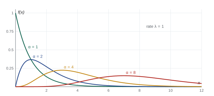
\(X\) has the gamma distribution with shape \(\alpha > 0\) and rate \(\lambda > 0\) if

It integrates to 1 by the substitution \(u = \lambda x\) and the definition of \(\Gamma\). The same substitution gives \(E[X^k] = \Gamma(\alpha + k)/(\Gamma(\alpha)\lambda^k)\), so \(E[X] = \alpha/\lambda\) and \(\operatorname{Var}(X) = \alpha/\lambda^2\). With \(\alpha = 1\) the gamma is the exponential. When \(\alpha = n\) is an integer, the gamma is the distribution of the sum of \(n\) independent exponential waiting times with rate \(\lambda\), sometimes called the Erlang distribution, which lesson 10 proves with moment generating functions. It is the waiting time until the \(n\)th event of a process with constant rate, such as the time until the third claim on a policy or the third failure in a system with two spares. Gamma distributions are also popular for claim amounts and rainfall totals, because their shape parameter gives flexible right skewness.

There is a neat link with the Poisson. If events occur at rate \(\lambda\) with independent exponential gaps, the \(n\)th event happens after time \(t\) exactly when fewer than \(n\) events have happened by \(t\). The number by time \(t\) is Poisson with mean \(\lambda t\), so \(P(\text{Gamma}(n, \lambda) > t) = \sum_{k=0}^{n-1}e^{-\lambda t}(\lambda t)^k/k!\). The two families describe the same process, one counting events in a fixed time and the other timing a fixed number of events.

The normal distribution

\(Z\) has the standard normal distribution if its density is

To see that it integrates to 1, let \(I = \int e^{-z^2/2}\,dz\). Then \(I^2 = \iint e^{-(x^2 + y^2)/2}\,dx\,dy\), and in polar coordinates this is \(\int_0^{2\pi}\int_0^\infty e^{-r^2/2}r\,dr\,d\theta = 2\pi\), so \(I = \sqrt{2\pi}\). This trick, squaring an integral to make it two-dimensional, is due to Poisson and is one of the prettiest in calculus. By symmetry \(E[Z] = 0\), and integrating by parts gives \(E[Z^2] = 1\), so \(\operatorname{Var}(Z) = 1\).

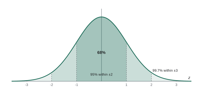
The general normal \(X \sim N(\mu, \sigma^2)\) is \(X = \mu + \sigma Z\), with density \(f(x) = \frac{1}{\sigma\sqrt{2\pi}}e^{-(x - \mu)^2/(2\sigma^2)}\), mean \(\mu\) and variance \(\sigma^2\). Every normal probability reduces to the standard normal cdf \(\Phi\): \(P(X \le x) = \Phi((x - \mu)/\sigma)\). The function \(\Phi\) has no elementary formula and is computed numerically; Python provides it through the error function, \(\Phi(z) = \frac12(1 + \operatorname{erf}(z/\sqrt2))\). Three numbers are worth memorizing: about 68%, 95% and 99.7% of a normal distribution lies within 1, 2 and 3 standard deviations of the mean. Compare these with Chebyshev's guarantees of 0%, 75% and 89%.

Normal distributions are closed under linear combinations of independent variables: if \(X \sim N(\mu_1, \sigma_1^2)\) and \(Y \sim N(\mu_2, \sigma_2^2)\) are independent, then \(aX + bY \sim N(a\mu_1 + b\mu_2, a^2\sigma_1^2 + b^2\sigma_2^2)\). Lesson 10 proves this with generating functions. This closure, together with the central limit theorem, is why the normal distribution is everywhere in statistics. It was de Moivre who first found the normal curve, in 1733, as an approximation to the binomial; Gauss later derived it as the law of measurement errors, which is why it is often called Gaussian.

The beta distribution

\(X\) has the beta distribution with parameters \(a, b > 0\) if

Its mean is \(a/(a + b)\) and its variance \(ab/((a + b)^2(a + b + 1))\). With \(a = b = 1\) it is the uniform on \((0, 1)\). Beta densities model proportions: the fraction of a day a machine is busy, the share of votes a candidate receives, the unknown success probability of a treatment. They are also the distributions of order statistics of uniform samples: the \(k\)th smallest of \(n\) independent uniforms on \((0, 1)\) is \(\text{Beta}(k, n - k + 1)\). In Bayesian statistics the beta is the natural prior for a binomial probability, because a beta prior updated with binomial data gives a beta posterior, a fact STAT-252 uses.

Weibull and lognormal

The Weibull distribution with shape \(k > 0\) and scale \(\theta > 0\) has survival function \(S(t) = \exp(-(t/\theta)^k)\) for \(t \ge 0\) and hazard \(h(t) = (k/\theta)(t/\theta)^{k-1}\). Its hazard increases for \(k > 1\), decreases for \(k < 1\) and is constant for \(k = 1\), the exponential. That flexibility makes it the standard model in reliability engineering for the lifetimes of bearings, insulation, wind turbine components and many other parts, and it also appears as the distribution of the weakest link in a chain of many components, a result from extreme value theory.

\(X\) is lognormal if \(\ln X\) is normal: \(X = e^{\mu + \sigma Z}\). Its mean is \(e^{\mu + \sigma^2/2}\), larger than its median \(e^\mu\), and it has a long right tail. Lognormal distributions arise when a quantity is the product of many small independent factors, by applying the central limit theorem to the logarithm. Incomes, particle sizes, the sizes of cities, stock prices over a fixed horizon and many insurance claim sizes are roughly lognormal. Because \(E[X]\) depends on \(\sigma^2\), averages of lognormal data are sensitive to the spread, and the mean claim on a book of business is driven by its largest claims.

Computing with continuous distributions

The code below uses only the standard library. It computes normal probabilities through the error function, checks the 68–95–99.7 rule, finds the cereal-box setting by bisection on \(\Phi\), verifies the gamma–Poisson identity, and simulates the gamma as a sum of exponentials and a beta as an order statistic of uniforms.

import math, random
from statistics import mean, pvariance

Phi = lambda z: 0.5 * (1 + math.erf(z / math.sqrt(2)))
for k in (1, 2, 3):
    print(f"P(|Z| < {k}) = {Phi(k) - Phi(-k):.4f}")

def z_quantile(q, lo=-10.0, hi=10.0):
    for _ in range(80):
        mid = (lo + hi) / 2
        lo, hi = (mid, hi) if Phi(mid) < q else (lo, mid)
    return (lo + hi) / 2
z01 = z_quantile(0.01)
print(f"underweight at mean 505: {Phi((500 - 505) / 4):.4f};  z_0.01 = {z01:.4f};  mean for 1%: {500 - 4 * z01:.2f}")

# gamma(3, rate 2): P(X > 1.5) from the Poisson formula, and by simulation as a sum of exponentials
lam, n, t = 2.0, 3, 1.5
exact = sum(math.exp(-lam * t) * (lam * t) ** k / math.factorial(k) for k in range(n))
rng = random.Random(251)
g = [sum(rng.expovariate(lam) for _ in range(n)) for _ in range(100_000)]
print(f"Gamma(3, 2): P(X > 1.5) exact {exact:.4f}, simulated {sum(x > t for x in g) / len(g):.4f}")
print(f"  mean {mean(g):.4f} (1.5), variance {pvariance(g):.4f} (0.75)")

# second smallest of 5 uniforms is Beta(2, 4): mean 1/3, variance 2/63
b = [sorted(rng.random() for _ in range(5))[1] for _ in range(100_000)]
print(f"Beta(2,4) via order statistic: mean {mean(b):.4f} (0.3333), var {pvariance(b):.5f} ({2/63:.5f})")

# lognormal: mean exceeds median
ln = [math.exp(rng.gauss(0, 1)) for _ in range(200_000)]
print(f"lognormal(0,1): mean {mean(ln):.3f} (e^0.5 = {math.exp(0.5):.3f}), median {sorted(ln)[100_000]:.3f} (1)")

P(|Z| < 1) = 0.6827
P(|Z| < 2) = 0.9545
P(|Z| < 3) = 0.9973
underweight at mean 505: 0.1056;  z_0.01 = -2.3263;  mean for 1%: 509.31
Gamma(3, 2): P(X > 1.5) exact 0.4232, simulated 0.4241
  mean 1.5042 (1.5), variance 0.7571 (0.75)
Beta(2,4) via order statistic: mean 0.3330 (0.3333), var 0.03167 (0.03175)
lognormal(0,1): mean 1.656 (e^0.5 = 1.649), median 1.006 (1)

Relationships among the families

The distributions of this lesson and the last form a connected web. The exponential is a gamma with shape 1 and a Weibull with shape 1. A sum of independent exponentials is gamma. The Poisson counts events whose gaps are exponential. The uniform is a beta with \(a = b = 1\), and uniform order statistics are beta. The binomial and Poisson are approximately normal when their means are large, by the central limit theorem. The lognormal is the exponential of a normal, and the chi-square of STAT-252 is a gamma with rate 1/2. Knowing these links means you do not have to memorize each distribution separately; you can derive facts about one from facts about another.

The value of Gamma(1/2) and the normal constant

The gamma function at one half connects the gamma family to the normal distribution. Substituting \(x = u^2/2\), so \(dx = u\,du\), in the definition gives

The last integral is half of \(\int_{-\infty}^\infty e^{-u^2/2}\,du = \sqrt{2\pi}\), a fact proved in lesson 10 with polar coordinates. So \(\Gamma(1/2) = \sqrt{2} \cdot \sqrt{2\pi}/2 = \sqrt{\pi}\). With the recursion \(\Gamma(\alpha + 1) = \alpha\Gamma(\alpha)\) this gives \(\Gamma(3/2) = \sqrt{\pi}/2\) and \(\Gamma(5/2) = 3\sqrt{\pi}/4\). The same calculation shows that the square of a standard normal has the gamma distribution with shape \(1/2\) and rate \(1/2\), the chi-squared distribution with one degree of freedom.

Worked example: standardizing in practice

Two facts make standardization reliable. First, if \(X \sim N(\mu, \sigma^2)\) then \((X - \mu)/\sigma\) is exactly standard normal, which follows from the linear change-of-variable rule; so one table, or one function such as Python's NormalDist().cdf, serves every normal distribution. Second, symmetry gives \(\Phi(-z) = 1 - \Phi(z)\), so tables need only list positive values. Real exam scores are bounded and slightly skewed, so the normal model is an approximation; it is usually good near the middle of the distribution and less reliable in the extreme tails, where decisions such as scholarships are often made.

Many Canadian growth charts, measurement standards and manufacturing tolerances use the same idea. A machine that fills 500 mL bottles with standard deviation 4 mL puts about 0.6% of bottles below 490 mL, since \(\Phi(-2.5) \approx 0.0062\). Raising the target mean to 502 mL cuts this to \(\Phi(-3) \approx 0.0013\), at the cost of 2 mL more product per bottle. Choosing the target is a trade-off between the cost of overfilling and the cost of underweight product, and the normal model makes that trade-off quantitative.

Why uniform order statistics are beta

The fact that uniform order statistics are beta has a short heuristic derivation. Draw \(n\) independent uniforms on \((0, 1)\) and let \(U_{(k)}\) be the \(k\)th smallest. For \(U_{(k)}\) to lie in a small interval \([x, x + dx]\), one of the \(n\) values must fall in that interval, \(k - 1\) of the others below \(x\) and \(n - k\) above. Counting the ways to assign the roles gives the density \(\frac{n!}{(k - 1)!\,(n - k)!}x^{k - 1}(1 - x)^{n - k}\), which is the beta density with \(a = k\) and \(b = n - k + 1\), since \(\Gamma(m) = (m - 1)!\). Its mean is \(a/(a + b) = k/(n + 1)\): the \(n\) sorted uniforms split the interval into \(n + 1\) gaps of equal expected length \(1/(n + 1)\). This is the reason plotting positions such as \(k/(n + 1)\) are used when comparing sorted data with a theoretical distribution, and it is how flood frequency analysts assign return periods to the largest floods on record: the largest of 50 annual floods is assigned an exceedance probability of about \(1/51\) per year.