
STAT-151 · Lesson 9 of 12 · 25 min
Categorical data analysis
Many scientific outcomes are categories rather than measurements: a seed germinates or does not, a patient recovers or does not, a fruit fly has red, white or brown eyes, a bird is found in forest, wetland or grassland. Data of this kind are summarized as counts, and the questions are about proportions and associations. This lesson covers inference for one and two proportions, the chi-square tests for goodness of fit and for association in two-way tables, Fisher’s exact test for small samples, and the relative risk and odds ratio, the effect sizes used throughout epidemiology and clinical research.
Inference for one proportion
Lesson 6 gave confidence intervals for a single proportion, recommending the Wilson or exact interval for small samples. The corresponding test of H₀: p = p₀ uses the standard error under the null hypothesis, √(p₀(1 − p₀)/n), giving z = (p̂ − p₀)/SE, or an exact binomial test, which scipy provides as stats.binomtest. The germination example in lesson 5 was a test of this kind.
Comparing two proportions
To compare two proportions, such as the infection rate in vaccinated and unvaccinated animals, the natural estimate is the difference p̂₁ − p̂₂. Its standard error for a confidence interval is √(p̂₁(1 − p̂₁)/n₁ + p̂₂(1 − p̂₂)/n₂). For a test of H₀: p₁ = p₂, the standard error uses the pooled proportion p̂ = (x₁ + x₂)/(n₁ + n₂), because under H₀ the two groups share one proportion.
Returning to the invented survey of 1,000 trees from lesson 3, 90 of 300 trees near salted roads had the fungal disease (p̂₁ = 0.30), compared with 70 of 700 trees away from roads (p̂₂ = 0.10).
import numpy as np
from scipy import stats
x1, n1, x2, n2 = 90, 300, 70, 700        # invented tree survey from lesson 3
p1, p2 = x1/n1, x2/n2
pool = (x1 + x2)/(n1 + n2)
z = (p1 - p2)/np.sqrt(pool*(1 - pool)*(1/n1 + 1/n2))
se = np.sqrt(p1*(1 - p1)/n1 + p2*(1 - p2)/n2)
print(f"p1 = {p1:.3f}, p2 = {p2:.3f}, difference = {p1 - p2:.3f}")
print(f"z = {z:.2f}, two-sided p = {2*stats.norm.sf(abs(z)):.2g}")
print(f"95% CI for the difference: {p1 - p2 - 1.96*se:.3f} to {p1 - p2 + 1.96*se:.3f}")p1 = 0.300, p2 = 0.100, difference = 0.200 z = 7.91, two-sided p = 2.7e-15 95% CI for the difference: 0.144 to 0.256
The difference of 20 percentage points is far too large to be explained by chance: the p-value is minute and the interval excludes zero by a wide margin. As lesson 3 stressed, this is an observational survey, so the association does not by itself show that salt causes disease.
Relative risk and odds ratio
A difference in proportions is one effect size. Two others are common in health and life sciences. The relative risk (RR), or risk ratio, divides the two proportions: here 0.30/0.10 = 3.0, so trees near roads were three times as likely to be diseased. The odds of an event are p/(1 − p), and the odds ratio (OR) compares odds: (0.30/0.70)/(0.10/0.90) = 3.86.
| Diseased | Healthy | Total | |
|---|---|---|---|
| Near road | a = 90 | b = 210 | 300 |
| Away from road | c = 70 | d = 630 | 700 |
When the outcome is rare (under about 10 percent in both groups), the odds ratio and relative risk are similar. When it is common, the odds ratio exaggerates the relative risk, and reports that describe an odds ratio of 3.86 as “nearly four times the risk” are wrong. Why use odds ratios at all? In case–control studies, which sample people with and without a disease and look back at their exposures, the proportion of cases is fixed by the design, so risks cannot be estimated, but the odds ratio can. Odds ratios are also the natural output of logistic regression, an extension of the regression methods of lessons 10 and 11 to binary outcomes.
Confidence intervals for both ratios are computed on the log scale, where the sampling distribution is closer to normal, and then back-transformed. For the odds ratio, the standard error of log(OR) is √(1/a + 1/b + 1/c + 1/d).
import numpy as np
a, b, c, d = 90, 210, 70, 630
rr = (a/(a + b))/(c/(c + d))
se_log_rr = np.sqrt(1/a - 1/(a + b) + 1/c - 1/(c + d))
odds_ratio = (a*d)/(b*c)
se_log_or = np.sqrt(1/a + 1/b + 1/c + 1/d)
for name, est, se in [("relative risk", rr, se_log_rr), ("odds ratio", odds_ratio, se_log_or)]:
    lo, hi = np.exp(np.log(est) - 1.96*se), np.exp(np.log(est) + 1.96*se)
print(f"{name:13s} = {est:.2f}, 95% CI {lo:.2f} to {hi:.2f}")relative risk = 3.00, 95% CI 2.26 to 3.98 odds ratio = 3.86, 95% CI 2.72 to 5.47
The chi-square goodness-of-fit test
Sometimes a theory predicts the proportions in several categories, and the question is whether observed counts fit. Gregor Mendel’s pea experiments are the classic case: a cross between two plants heterozygous for seed shape and color predicts a 9 : 3 : 3 : 1 ratio of the four phenotypes. The chi-square goodness-of-fit test compares observed counts O with the counts E expected under H₀.
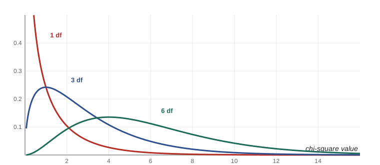
Each term measures how far one category departs from expectation, relative to the expected count. If H₀ is true, the statistic approximately follows a chi-square distribution with k − 1 degrees of freedom, where k is the number of categories (one fewer if a parameter has been estimated from the data). Large values indicate poor fit. The approximation is reliable when all expected counts are at least 5.
Worked problem
A dihybrid cross
Mendel reported 315 round yellow, 108 round green, 101 wrinkled yellow and 32 wrinkled green seeds, a total of 556. Do these fit the 9 : 3 : 3 : 1 ratio?
Show solution
- Expected counts: 556 × 9/16 = 312.75, 556 × 3/16 = 104.25 (twice), 556 × 1/16 = 34.75.
- χ² = (315 − 312.75)²/312.75 + (108 − 104.25)²/104.25 + (101 − 104.25)²/104.25 + (32 − 34.75)²/34.75 ≈ 0.016 + 0.135 + 0.101 + 0.218 = 0.47.
- df = 4 − 1 = 3; P(χ²₃ ≥ 0.47) ≈ 0.93.
Answer: The fit is excellent; the data give no evidence against the 9 : 3 : 3 : 1 ratio. In 1936 R. A. Fisher pointed out that Mendel’s data as a whole fitted his ratios rather better than chance would usually allow, a puzzle still debated by historians of science.
from scipy import stats
observed = [315, 108, 101, 32]                       # Mendel (1866)
expected = [556*9/16, 556*3/16, 556*3/16, 556*1/16]
chi2, p = stats.chisquare(observed, expected)
print(f"chi-square = {chi2:.3f}, df = 3, p = {p:.3f}")chi-square = 0.470, df = 3, p = 0.925
The chi-square test of independence
For a two-way table cross-classifying units by two categorical variables, the chi-square test of independence asks whether the variables are associated. Under H₀ of independence, the expected count in each cell is (row total × column total)/grand total, which is just the multiplication rule for independent events from lesson 3. The statistic is again Σ(O − E)²/E, with (r − 1)(c − 1) degrees of freedom for a table with r rows and c columns.
import numpy as np
from scipy import stats

# Invented: habitat use by three bird species (counts of sightings)
table = np.array([[42, 18, 10],    # warbler: forest, wetland, grassland
                  [15, 35, 12],    # rail
                  [20, 14, 38]])   # sparrow
res = stats.chi2_contingency(table)
print(f"chi-square = {res.statistic:.1f}, df = {res.dof}, p = {res.pvalue:.2g}")
print("expected counts:")
print(np.round(res.expected_freq, 1))
resid = (table - res.expected_freq)/np.sqrt(res.expected_freq)
print("standardized residuals (O - E)/sqrt(E):")
print(np.round(resid, 1))chi-square = 50.6, df = 4, p = 2.7e-10 expected counts: [[26.4 23. 20.6] [23.4 20.4 18.2] [27.2 23.6 21.2]] standardized residuals (O - E)/sqrt(E): [[ 3. -1. -2.3] [-1.7 3.2 -1.5] [-1.4 -2. 3.7]]
A significant chi-square says that the variables are associated but not how. The standardized residuals, (O − E)/√E, show which cells contribute most; values beyond about ±2 mark cells with notably more or fewer observations than independence predicts. Here warblers are over-represented in forest, rails in wetland and sparrows in grassland, which is the ecological story.
For a 2 × 2 table, the chi-square test of independence is equivalent to the two-proportion z test (χ² = z²). By default, scipy applies Yates’s continuity correction to 2 × 2 tables, which makes the test slightly more conservative; the correction is controversial and is unnecessary when expected counts are large.
Fisher’s exact test
When expected counts are small, the chi-square approximation is unreliable. Fisher’s exact test computes the probability of the observed table, and of all more extreme tables with the same row and column totals, exactly, using the hypergeometric distribution built from the binomial coefficients of lesson 3. Fisher devised it to analyze a famous experiment in which a colleague, Muriel Bristol, claimed she could tell whether milk or tea had been poured into the cup first.
from scipy import stats
# Invented: frogs infected with chytrid fungus in two ponds
#            infected  not infected
table = [[7, 3],      # pond A
         [2, 9]]      # pond B
res = stats.fisher_exact(table)
print(f"sample odds ratio = {res.statistic:.1f}, Fisher exact p = {res.pvalue:.4f}")
chi = stats.chi2_contingency(table)
print(f"smallest expected count = {chi.expected_freq.min():.1f} (below 5, so prefer Fisher)")sample odds ratio = 10.5, Fisher exact p = 0.0300 smallest expected count = 4.3 (below 5, so prefer Fisher)
Assumptions and pitfalls
All of these tests assume that each unit contributes to exactly one cell and that units are independent. Counting the same animal several times, or treating the many seeds from one plant as independent, inflates the effective sample size, just like pseudoreplication with measurements. Percentages must always be converted back to counts before a chi-square test: the test depends on the actual numbers, and 30 percent of 10 is very different evidence from 30 percent of 1,000.
Associations in tables can also reverse when a third variable is ignored, a phenomenon called Simpson’s paradox. In a well-known real example, the 1973 graduate admissions at the University of California, Berkeley appeared to favor men overall, but within most departments women were admitted at similar or higher rates; women had applied more often to departments with low admission rates. The lesson for scientists is to think about confounding variables and, where possible, to stratify the analysis.
| Situation | Method |
|---|---|
| One proportion against a stated value | Exact binomial test; Wilson or exact interval |
| Two proportions, large samples | Two-proportion z test or chi-square; interval for difference, RR or OR |
| Observed counts against theoretical proportions | Chi-square goodness-of-fit test |
| Association in an r × c table, expected counts at least 5 | Chi-square test of independence with standardized residuals |
| 2 × 2 table with small expected counts | Fisher’s exact test |
| Paired binary outcomes (same subjects twice) | McNemar’s test |
Common mistakes
MistakeRun a chi-square test on percentages.
InsteadChi-square tests must use the actual counts.
MistakeDescribe an odds ratio of 3.9 as nearly four times the risk.
InsteadWhen the outcome is common, the odds ratio overstates the relative risk; report the RR, or describe the OR as a ratio of odds.
MistakeUse the chi-square test when several expected counts are below 5.
InsteadUse Fisher’s exact test, or combine categories if that makes scientific sense.
MistakeA significant chi-square test shows which categories differ.
InsteadIt shows only that an association exists; examine standardized residuals or proportions to see where.
MistakeCount each observation of the same animal as a separate unit.
InsteadEach independent unit must contribute once; repeated observations of the same unit need methods for dependent data.
MistakeAn association in the combined table holds within every subgroup.
InsteadSimpson’s paradox shows that aggregating can reverse associations; consider confounders.
Summary and key terms
- Categorical data are summarized as counts; inference concerns proportions and associations.
- Two proportions can be compared by their difference, relative risk or odds ratio, each with a confidence interval.
- Odds ratios approximate relative risks only for rare outcomes, but are the natural measure in case–control studies.
- The chi-square goodness-of-fit test compares observed counts with those predicted by a theory.
- The chi-square test of independence compares observed cell counts with those expected if the variables were unrelated.
- Standardized residuals show which cells drive an association.
- Fisher’s exact test is used for small 2 × 2 tables; all methods require independent units counted once.
- relative risk
- The ratio of the probabilities of an outcome in two groups.
- odds
- The ratio of the probability of an event to the probability that it does not occur.
- odds ratio
- The ratio of the odds of an outcome in two groups.
- case–control study
- An observational study that samples people with and without an outcome and compares their past exposures.
- goodness-of-fit test
- A test of whether observed counts match proportions specified by a hypothesis.
- test of independence
- A test of whether two categorical variables are associated in a two-way table.
- expected count
- The count predicted for a cell under the null hypothesis.
- standardized residual
- The quantity (O − E)/√E, showing how much a cell departs from expectation.
- Fisher’s exact test
- An exact test for association in a 2 × 2 table, suitable for small samples.
- Simpson’s paradox
- A reversal of an association when data from subgroups are combined.
Practice problems
Work each problem on paper first, then reveal the answer to check.
In 80 treated plants, 20 are diseased; in 80 controls, 36 are. Find the difference in proportions.
Show answer
0.25 − 0.45 = −0.20.
For the plants above, find the relative risk of disease for treated versus control.
Show answer
0.25/0.45 = 0.56.
For the same data, find the odds ratio.
Show answer
(20 × 44)/(60 × 36) = 880/2160 = 0.41.
Why are the RR and OR different in the plant example?
Show answer
The outcome is common (25 to 45 percent), so the odds ratio departs from the relative risk.
A die is rolled 120 times. What is the expected count for each face if it is fair?
Show answer
20.
What are the degrees of freedom for a chi-square test of independence on a 3 × 4 table?
Show answer
(3 − 1)(4 − 1) = 6.
In a 2 × 2 table the row totals are 50 and 150 and a column total is 40. Find the expected count in the first cell of that column.
Show answer
50 × 40/200 = 10.
A 2 × 2 table has expected counts of 2.5, 3.5, 7.5 and 10.5. Which test should be used?
Show answer
Fisher’s exact test.
A standardized residual is +3.1. Interpret it.
Show answer
That cell has many more observations than expected under independence.
Explain Simpson’s paradox in one sentence.
Show answer
An association seen in combined data can disappear or reverse within subgroups because of a confounding variable.
Lesson quiz · 5 questions
Score 60% or more to complete this lesson.
Create a free account to save your progress, take quizzes and earn a certificate.