Sampling distributions and the central limit theorem

If two research groups each measure the mean height of 30 randomly chosen seedlings from the same greenhouse, they will not get exactly the same answer. Each sample mean is a random variable: its value depends on which seedlings happen to be chosen. The sampling distribution of a statistic is the distribution of values it would take over all possible samples of the same size from the same population. Understanding sampling distributions is the key step from describing data to drawing conclusions from them, because every confidence interval and hypothesis test in this course is built on one. This lesson uses simulation to show how sampling distributions behave and introduces the central limit theorem, one of the most important results in all of mathematics for science.

Simulating a sampling distribution

In real research we have one sample and cannot see the sampling distribution directly. In a computer we can create a population, draw thousands of samples from it, and look at how a statistic varies. The simulation below uses an invented population of 100,000 fish lengths, then draws many samples of size 25 and records the mean of each.

import numpy as np
rng = np.random.default_rng(151)

# An invented population: lengths (cm) of 100,000 lake trout
population = rng.normal(48, 9, 100_000)
mu, sigma = population.mean(), population.std()

means = np.array([rng.choice(population, 25, replace=False).mean() for _ in range(5000)])
print(f"population mean {mu:.2f} cm, population SD {sigma:.2f} cm")
print(f"mean of 5,000 sample means      = {means.mean():.2f} cm")
print(f"SD of sample means (simulated)  = {means.std(ddof=1):.3f} cm")
print(f"sigma / sqrt(25) (theory)        = {sigma/np.sqrt(25):.3f} cm")
print(f"middle 95% of sample means: {np.percentile(means, 2.5):.2f} to {np.percentile(means, 97.5):.2f} cm")

population mean 48.04 cm, population SD 9.01 cm
mean of 5,000 sample means      = 47.99 cm
SD of sample means (simulated)  = 1.789 cm
sigma / sqrt(25) (theory)        = 1.802 cm
middle 95% of sample means: 44.41 to 51.47 cm

Three facts emerge, and they hold generally. First, the sample means are centered on the population mean: the sample mean is an unbiased estimator of μ. Second, the sample means vary much less than individual fish: their standard deviation is σ/√n, the standard error introduced in lesson 1. Third, 95 percent of sample means fall within about two standard errors of μ, as the normal distribution predicts.

The mean and standard error of the sample mean

These facts follow directly from the rules for expected values and variances in lesson 4. If X₁, …, Xₙ are independent observations from a population with mean μ and standard deviation σ, then the sample mean has expected value μ and variance σ²/n.

The derivation is short. The sum of n independent observations has mean nμ and, because variances of independent quantities add, variance nσ². Dividing the sum by n divides the mean by n and the variance by n². The independence assumption matters: if observations are positively correlated, as with subsamples from the same experimental unit, the true variance of the mean is larger than σ²/n, which is the mathematical reason pseudoreplication is so dangerous.

In practice σ is unknown and is replaced by the sample standard deviation s, giving the estimated standard error s/√n. This substitution adds a little extra uncertainty, which the t distribution of lesson 6 accounts for.

The central limit theorem

The fish lengths in the first simulation were normal, so it is not surprising that their means were normal too: sums and averages of normal variables are exactly normal. The remarkable fact is that sample means are approximately normal even when the original data are not. The central limit theorem (CLT) states that, for independent observations from any population with finite variance, the sampling distribution of the mean approaches a normal distribution as the sample size grows.

How large is large? It depends on how far the population is from normal. For roughly symmetric populations, samples of 10 or 15 give nearly normal means. For moderately skewed populations, 30 is a common rule of thumb. For very skewed populations, such as the lognormal contaminant concentrations of lesson 4 or counts with many zeros, much larger samples may be needed. The simulation below shows the CLT at work on a strongly right-skewed population.

import numpy as np
from scipy import stats
rng = np.random.default_rng(1515)

# A strongly right-skewed population: exponential waiting times with mean 10 minutes
def skew(x):
    return stats.skew(x)

print("Population skewness (exponential) = 2.00")
for n in (1, 5, 30, 100):
    means = rng.exponential(10, size=(20_000, n)).mean(axis=1)
    se = 10/np.sqrt(n)
    low = np.mean(means < 10 - 1.96*se)
    high = np.mean(means > 10 + 1.96*se)
    print(f"n = {n:3d}: skewness of means = {skew(means):5.2f}; "
          f"below -1.96 SE: {low:.3f}, above +1.96 SE: {high:.3f}")

Population skewness (exponential) = 2.00
n =   1: skewness of means =  2.02; below -1.96 SE: 0.000, above +1.96 SE: 0.052
n =   5: skewness of means =  0.86; below -1.96 SE: 0.000, above +1.96 SE: 0.043
n =  30: skewness of means =  0.35; below -1.96 SE: 0.015, above +1.96 SE: 0.033
n = 100: skewness of means =  0.20; below -1.96 SE: 0.019, above +1.96 SE: 0.031

Single observations from an exponential distribution have skewness 2; the means of 30 have skewness close to 0.35, and the means of 100 are nearly symmetric. The tail shares tell the same story. For a normal distribution, 2.5 percent of values lie more than 1.96 standard deviations below the mean and 2.5 percent lie the same distance above it. For single exponential observations, no value can fall that far below the mean (waiting times cannot be negative), while about 5 percent lie that far above it. The overall 95 percent coverage looks right only by coincidence: the two tails are badly unbalanced. As n grows, both tail shares move toward 0.025, which shows that the normal approximation can be poor for individual skewed observations even though it works well for means.

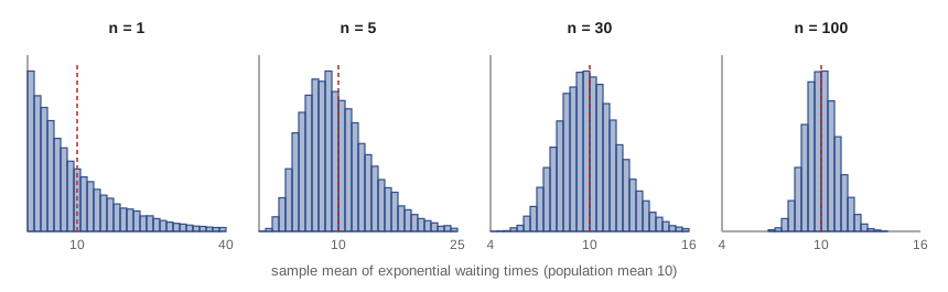
The CLT explains why the normal distribution is so common in nature as well as in statistics. Quantities that result from the sum of many small, independent effects, such as height, which depends on hundreds of genes and many environmental influences, tend to be approximately normal. BIOL-201 uses exactly this argument to explain why quantitative traits are bell-shaped.

The sampling distribution of a proportion

A sample proportion, p̂ = X/n, where X is the number of successes in n trials, is a special kind of mean: it is the mean of n observations each equal to 1 (success) or 0 (failure). From the binomial distribution of lesson 4, p̂ has mean p and standard error √(p(1 − p)/n). By the CLT, p̂ is approximately normal when n is large; a common guideline is that np and n(1 − p) should both be at least 10.

from scipy import stats
n, p, x = 200, 0.85, 160
se = (p*(1 - p)/n) ** 0.5
z = (x/n - p) / se
print(f"normal approximation: z = {z:.2f}, P(p-hat <= 0.80) = {stats.norm.cdf(z):.4f}")
print(f"exact binomial:       P(X <= 160)      = {stats.binom.cdf(x, n, p):.4f}")

normal approximation: z = -1.98, P(p-hat <= 0.80) = 0.0238
exact binomial:       P(X <= 160)      = 0.0335

The normal approximation gives about 0.024 and the exact binomial calculation about 0.034. Both lead to the same practical conclusion, but the difference is a reminder that the approximation treats a discrete count as if it were continuous. With modern software, exact binomial probabilities are easy to compute and are preferable for small samples or proportions near 0 or 1, but the normal approximation remains useful for understanding and for quick calculations.

Sampling distributions of other statistics

Every statistic has a sampling distribution. The sample median, the standard deviation, a correlation coefficient and a regression slope all vary from sample to sample. Some have neat formulas; for others, statisticians use simulation. A useful comparison is between the mean and the median: for normal data, the median is also unbiased but has a standard error about 25 percent larger than the mean, so it is less efficient. For heavy-tailed data with occasional extreme values, the median can be more precise. This trade-off is one reason robust methods, introduced in lesson 2, are valuable.

import numpy as np
rng = np.random.default_rng(15105)
n, reps = 25, 20_000

normal = rng.normal(0, 1, size=(reps, n))
heavy = rng.standard_t(2, size=(reps, n))      # heavy-tailed data

for name, x in [("normal data", normal), ("heavy-tailed data", heavy)]:
    se_mean = x.mean(axis=1).std(ddof=1)
    se_median = np.median(x, axis=1).std(ddof=1)
    print(f"{name:18s}: SE(mean) = {se_mean:.3f}, SE(median) = {se_median:.3f}")

normal data       : SE(mean) = 0.200, SE(median) = 0.250
heavy-tailed data : SE(mean) = 0.730, SE(median) = 0.288

Why the sample standard deviation divides by n − 1

Simulation also shows why lesson 2 used n − 1 in the sample variance. If we divide the sum of squared deviations by n, the result is too small on average, because the deviations are measured from the sample mean, which is always closer to the data than the true mean is. Dividing by n − 1 removes this bias exactly for the variance.

import numpy as np
rng = np.random.default_rng(15106)
sigma2 = 4.0
samples = rng.normal(0, 2, size=(50_000, 5))     # small samples of 5 make the bias obvious
print(f"true variance = {sigma2}")
print(f"average of variance with divisor n     = {samples.var(axis=1, ddof=0).mean():.3f}")
print(f"average of variance with divisor n - 1 = {samples.var(axis=1, ddof=1).mean():.3f}")

true variance = 4.0
average of variance with divisor n     = 3.193
average of variance with divisor n - 1 = 3.992

With samples of five, dividing by n underestimates the variance by about 20 percent, a factor of (n − 1)/n = 0.8, while dividing by n − 1 is correct on average. The square root, s, is still slightly biased downward as an estimate of σ, but the bias is small and is usually ignored.

Bias, precision and good estimators

A good estimator is close to the parameter it estimates. Two properties describe closeness. Bias is the difference between the estimator’s average value and the parameter; an unbiased estimator is right on average. Precision is the opposite of variability: a precise estimator has a small standard error. The mean squared error combines both: MSE = bias² + variance. Ideally an estimator has low bias and high precision, like arrows clustered on the center of a target. Larger samples improve precision but cannot remove bias from a flawed design, the point made in lesson 1 about samples of trees along roads.