Describing data and measurement uncertainty

Before testing any hypothesis, a scientist must look at the data. Plotting and summarizing measurements reveals their shape, their typical values and how much they vary, and it exposes problems such as recording errors, outliers and instruments that drifted during a run. This lesson covers the tools for describing a single quantitative variable: graphs of distributions, measures of center and spread, robust alternatives that resist outliers, and the standard ways of reporting measurement uncertainty. STAT-235 treats these ideas for engineering data and quality control; here the emphasis is on laboratory and field measurements in the life and physical sciences.

Looking at distributions

The distribution of a variable describes which values occur and how often. The simplest graphical summary for a quantitative variable is the histogram, which divides the range of values into intervals called bins and draws a bar for the number (or proportion) of observations in each. A histogram shows the shape of a distribution: whether it is symmetric or skewed, whether it has one peak (unimodal) or several (multimodal), and whether there are gaps or unusual values.

Many biological and environmental variables are right-skewed: most values are small, with a long tail of larger ones. Concentrations of pollutants, bacterial counts, body masses across species and incomes all tend to be right-skewed because they cannot fall below zero but can be very large. Left-skewed distributions, with a long tail of small values, are less common; examples include the age at death in a wealthy country and exam scores on an easy test. Bimodal distributions often signal that two different groups have been mixed, such as the body lengths of male and female fish or of two age classes.

import numpy as np
rng = np.random.default_rng(151)

# Invented data: nitrate concentration (mg/L) in 60 well-water samples
nitrate = np.round(rng.lognormal(mean=1.2, sigma=0.8, size=60), 2)
print("First ten values:", nitrate[:10])

# A text histogram with bins of width 2 mg/L
counts, edges = np.histogram(nitrate, bins=np.arange(0, 16, 2))
for c, lo, hi in zip(counts, edges[:-1], edges[1:]):
    print(f"{lo:4.0f}-{hi:<4.0f} | {'#' * c}  ({c})")

First ten values: [0.68 1.34 1.34 9.16 0.88 7.44 3.69 2.83 4.81 0.86]
   0-2    | ####################  (20)
   2-4    | #############  (13)
   4-6    | #################  (17)
   6-8    | #####  (5)
   8-10   | ###  (3)
  10-12   | #  (1)
  12-14   | #  (1)

Most wells have nitrate below 6 mg/L, but a few have much higher values, producing a long right tail. Health Canada and the US Environmental Protection Agency both set a drinking water limit for nitrate expressed as nitrogen of 10 mg/L, so the few high values are the ones that matter most for public health. A summary that hid the tail would be misleading.

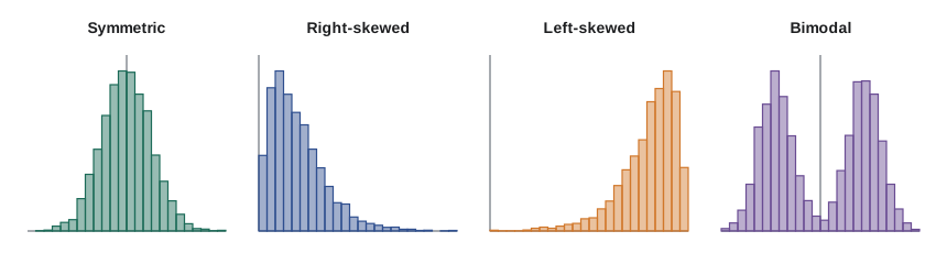
Other useful graphs include the dot plot, which shows every observation and is ideal for small samples; the stem-and-leaf plot, a quick paper-and-pencil display; and the box plot, described below, which is excellent for comparing several groups side by side. For small samples of fewer than about 20 values, showing every point is usually better than a histogram, whose appearance can depend heavily on the choice of bins.

Measures of center

The mean is the arithmetic average: the sum of the observations divided by their number. The median is the middle value when the observations are sorted, or the average of the two middle values when n is even. For a symmetric distribution, the mean and median are close. For a skewed distribution, the mean is pulled toward the long tail, because extreme values contribute their full size to the sum, while the median depends only on the order of the values.

Which measure to report depends on the question. The mean is the right summary when totals matter: the mean daily nitrate load times the number of days gives the total load delivered to a lake. The median better describes a typical value in skewed data: half the wells have nitrate below the median. Reporting both, along with a graph, is often the most informative choice. The mode, the most common value, is mainly useful for categorical data.

A trimmed mean compromises between the two by discarding a fixed percentage of the smallest and largest values before averaging. A 10 percent trimmed mean removes the lowest and highest 10 percent of observations. Trimmed means are used in some sports judging and in some economic indicators, such as the Bank of Canada’s CPI-trim measure of core inflation, because they resist the influence of a few extreme values.

Measures of spread

Two samples can have the same center but very different spread. The range, the difference between the largest and smallest values, is easy to compute but depends entirely on the two most extreme observations and grows with sample size. Better measures use all the data.

The variance is the average squared deviation from the mean, computed with n − 1 in the denominator for a sample, and the standard deviation is its square root, which returns the measure to the original units. The divisor n − 1, called the degrees of freedom, corrects for the fact that deviations are measured from the sample mean rather than the unknown population mean, which makes them slightly too small on average. STAT-252 proves this; here it is enough to know that software uses n − 1 by default for sample variances (numpy needs the argument ddof=1).

The quartiles split sorted data into four parts. The first quartile, Q1, has a quarter of the observations below it; the third quartile, Q3, has three-quarters below it; the median is the second quartile. The interquartile range (IQR), Q3 − Q1, is the spread of the middle half of the data. Like the median, it is resistant to extreme values. The five-number summary, minimum, Q1, median, Q3 and maximum, is the basis of the box plot.

import numpy as np
rng = np.random.default_rng(151)
nitrate = np.round(rng.lognormal(mean=1.2, sigma=0.8, size=60), 2)

mean, median = nitrate.mean(), np.median(nitrate)
sd = nitrate.std(ddof=1)
q1, q3 = np.percentile(nitrate, [25, 75])
iqr = q3 - q1
lo_fence, hi_fence = q1 - 1.5*iqr, q3 + 1.5*iqr
outliers = nitrate[(nitrate < lo_fence) | (nitrate > hi_fence)]

print(f"n = {nitrate.size}, mean = {mean:.2f}, median = {median:.2f} mg/L")
print(f"SD = {sd:.2f}, Q1 = {q1:.2f}, Q3 = {q3:.2f}, IQR = {iqr:.2f}")
print(f"Five-number summary: {nitrate.min():.2f}, {q1:.2f}, {median:.2f}, {q3:.2f}, {nitrate.max():.2f}")
print(f"1.5 x IQR fences: {lo_fence:.2f} and {hi_fence:.2f}; flagged values: {np.sort(outliers)}")
print(f"Samples above the 10 mg/L limit: {(nitrate > 10).sum()}")

n = 60, mean = 3.76, median = 3.20 mg/L
SD = 2.71, Q1 = 1.72, Q3 = 4.78, IQR = 3.06
Five-number summary: 0.43, 1.72, 3.20, 4.78, 12.47
1.5 x IQR fences: -2.88 and 9.38; flagged values: [11.12 12.47]
Samples above the 10 mg/L limit: 2

The mean is larger than the median, as expected for right-skewed data. The IQR rule flags the largest values as potential outliers. These are not errors; they are real wells with high nitrate, and they are the most important observations in the data set.

Box plots and comparing groups

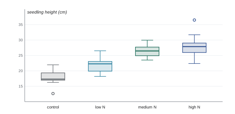
A box plot draws a box from Q1 to Q3 with a line at the median, and whiskers extending to the most extreme observations that lie within 1.5 × IQR of the box. Points beyond the whiskers are plotted individually. Box plots are compact enough to place several side by side, which makes them a standard way to compare groups, such as plant heights under different fertilizer treatments, before a formal analysis such as the ANOVA of lesson 12.

Outliers: investigate before acting

An outlier is an observation that lies far from the rest. The 1.5 × IQR rule and the rule of more than three standard deviations from the mean are common screening tools, but neither decides what to do. An outlier may be a recording error (a decimal point in the wrong place), an instrument failure, a sample from a different population (a contaminated vial), or a genuine and important extreme value. The correct response is to investigate: check laboratory notebooks, instrument logs and sample labels.

Values should be removed only when there is an independent reason to believe they are wrong, and the removal must be reported. Deleting inconvenient values because they weaken a result is a form of scientific misconduct. When a legitimate extreme value strongly influences a result, a good practice is to report the analysis with and without it, or to use robust methods, such as the median and IQR, or the rank-based tests of lesson 8, that are less sensitive to extremes.

Another robust measure of spread is the median absolute deviation (MAD), the median of the absolute deviations from the median. Multiplied by 1.4826, it estimates the standard deviation for normally distributed data but is barely affected by a few outliers.

import numpy as np
# Eight replicate absorbance readings of a standard, one mistyped (0.512 entered as 5.12)
x = np.array([0.508, 0.514, 0.511, 0.509, 0.516, 5.12, 0.513, 0.510])
clean = np.delete(x, 5)

def mad_sd(v):
    return 1.4826 * np.median(np.abs(v - np.median(v)))

for name, v in [("with typo", x), ("typo removed", clean)]:
    print(f"{name:12s}: mean {v.mean():.3f}, median {np.median(v):.4f}, "
          f"SD {v.std(ddof=1):.3f}, robust SD (MAD) {mad_sd(v):.4f}")

with typo   : mean 1.088, median 0.5120, SD 1.629, robust SD (MAD) 0.0037
typo removed: mean 0.512, median 0.5110, SD 0.003, robust SD (MAD) 0.0030

The mistyped value roughly doubles the mean and the standard deviation by a factor of several hundred, while the median and the MAD-based estimate hardly move. Robust summaries are an excellent first check: a large gap between the mean and median, or between the SD and the robust SD, is a sign that something needs investigating.

Linear transformations and standardized values

Changing units changes summaries in predictable ways. If every value is multiplied by a constant b and has a constant a added, as in converting °C to °F (b = 1.8, a = 32), the mean and median are transformed the same way, while the standard deviation and IQR are multiplied by |b| and are unaffected by a. A z-score expresses a value as the number of standard deviations it lies from the mean, z = (x − x̄)/s. Z-scores have no units, so they allow comparisons between variables measured on different scales, such as a fish that is unusually long and also unusually heavy for its age.

Measurement uncertainty and significant figures

Every measurement has uncertainty. Metrologists distinguish accuracy, how close a measurement is to the true value, from precision, how close repeated measurements are to each other. A balance that always reads 0.5 g too high is precise but inaccurate; its error is systematic and is corrected by calibration. Random scatter in repeated readings limits precision and is reduced by averaging. The international Guide to the Expression of Uncertainty in Measurement (GUM), used by national metrology institutes including the National Research Council of Canada and the US National Institute of Standards and Technology, distinguishes Type A uncertainties, evaluated statistically from repeated measurements, from Type B uncertainties, evaluated from other information such as calibration certificates and instrument specifications.

For repeated measurements, the uncertainty of the mean is usually reported as the standard error, s/√n, sometimes multiplied by a coverage factor of about 2 to give an interval with roughly 95 percent confidence, an idea made precise in lesson 6. Results should be reported with a number of digits that reflects their uncertainty: a mean of 12.34567 mg with a standard error of 0.2 mg should be reported as 12.3 ± 0.2 mg. Carrying extra digits through intermediate calculations and rounding only at the end avoids accumulating rounding errors.

Propagation of uncertainty

Scientists often calculate a result from several measured quantities, such as a concentration from a mass and a volume, or a growth rate from two lengths and a time. Propagation of uncertainty describes how the uncertainties of the inputs combine. For independent inputs and small uncertainties, the rules follow from the first-order Taylor approximation in MATH-100: for sums and differences, absolute uncertainties combine in quadrature (as the square root of the sum of squares); for products and quotients, relative uncertainties combine in quadrature. CHEM-101 applies these rules to laboratory chemistry.

import numpy as np
rng = np.random.default_rng(1514)

# Check the propagation formula by simulation (Monte Carlo)
m = rng.normal(0.2500, 0.0002, 200_000)     # g
V = rng.normal(0.2500, 0.0002, 200_000)     # L (0.2 mL)
c = m / V
print(f"Monte Carlo: c = {c.mean():.4f} g/L, standard uncertainty {c.std(ddof=1):.5f} g/L")
print(f"Formula:     standard uncertainty {1.000*np.sqrt((0.0002/0.25)**2 + (0.0002/0.25)**2):.5f} g/L")

Monte Carlo: c = 1.0000 g/L, standard uncertainty 0.00113 g/L
Formula:     standard uncertainty 0.00113 g/L

Monte Carlo simulation, which draws many random values of each input and computes the result for each, is a general alternative to the formulas. It handles non-linear functions and large uncertainties that the first-order formulas approximate poorly, and it is recommended in a supplement to the GUM for exactly those cases.