
ROB-420 · Lesson 4 of 12 · 29 min
Prediction and behavior planning
Perception tells an automated vehicle what is around it now. To drive well it must also anticipate what those road users will do next and decide what it should do in response: keep the lane or change, yield or go, nudge around a parked truck or wait. This lesson covers the prediction of other agents' motion and intent, and the behavior planning layer that chooses a maneuver. These two problems are tightly linked, because what others do depends on what the automated vehicle does, and the reverse. We look at physics-based and learned prediction, the idea of multimodal futures, interaction and game-theoretic thinking, and the long-running debate between rule-based and learned decision-making.
Why prediction is hard
A pedestrian standing at the curb may cross, wait or turn and walk along the sidewalk. A car in the next lane may hold its lane or cut in. A cyclist may swerve to avoid a pothole. These futures are uncertain and often multimodal: there are several distinct possibilities rather than one most likely path with small scatter. Averaging them produces nonsense, such as a predicted path that drives halfway between going straight and turning left. A good predictor outputs several possible trajectories with probabilities, and the planner must make a choice that is safe against the plausible ones, not just the most likely.
Prediction horizons are typically 3 to 8 seconds. Over the first second, physics dominates: a vehicle cannot change its velocity much. Beyond a few seconds, intent dominates: where the driver wants to go, what lane they are in, whether they have signaled, and how traffic around them is moving.
Physics-based prediction
The simplest predictors extrapolate current motion. A constant-velocity model assumes the agent continues at its present speed and heading; a constant-turn-rate-and-velocity model, CTRV, also continues its current turning. These work surprisingly well for one or two seconds and are a valuable baseline and fallback, but fail when agents follow the road, stop at signals or react to others.
Worked problem
Constant velocity versus a turning car
A car travels at 10 m/s with yaw rate 0.2 rad/s (it is turning left). Where does a constant-velocity model predict it after 3 s, and where does the CTRV model put it? Start at the origin heading along x.
Show solution
- Constant velocity: \( x = 30 \) m, \( y = 0 \).
- CTRV: \( v/\omega = 50 \) m, \( \omega t = 0.6 \) rad.
- \( x = 50 \sin 0.6 = 50 \times 0.565 = 28.2 \) m.
- \( y = -50(\cos 0.6 - 1) = 50 \times 0.175 = 8.7 \) m.
Answer: Constant velocity says (30, 0); CTRV says about (28.2, 8.7). The 8.7 m difference is more than two lanes, showing why turning must be modeled.
# Constant velocity vs constant turn rate prediction errors for a turning car
import numpy as np
rng = np.random.default_rng(3)
v, w, dt = 10.0, 0.2, 0.1
t = np.arange(0, 3.01, dt)
# truth: car turns at 0.2 rad/s with slight speed noise
x_true = (v / w) * np.sin(w * t)
y_true = -(v / w) * (np.cos(w * t) - 1)
x_cv, y_cv = v * t, np.zeros_like(t)
w_est = w + rng.normal(0, 0.02)              # noisy yaw-rate estimate
x_ct = (v / w_est) * np.sin(w_est * t)
y_ct = -(v / w_est) * (np.cos(w_est * t) - 1)
for T in (1.0, 2.0, 3.0):
    k = int(round(T / dt))
    e_cv = np.hypot(x_cv[k] - x_true[k], y_cv[k] - y_true[k])
    e_ct = np.hypot(x_ct[k] - x_true[k], y_ct[k] - y_true[k])
print(f"t={T:.0f} s CV error {e_cv:5.2f} m CTRV error {e_ct:5.2f} m")t=1 s CV error 1.00 m CTRV error 0.20 m t=2 s CV error 3.98 m CTRV error 0.81 m t=3 s CV error 8.91 m CTRV error 1.81 m
Map-aware and learned prediction
Vehicles mostly follow lanes. Map-aware predictors use the HD map from Lesson 3 to enumerate the lanes an agent could take, such as continuing straight, turning right or changing lanes, and then estimate the probability of each based on position, speed, heading, turn signals and history. Each hypothesis becomes a trajectory along its lane path with a speed profile. This approach is interpretable and handles common cases well.
Learned predictors, trained on millions of recorded interactions, take as input the recent history of all nearby agents and a representation of the map, often as a graph of lane segments or a rasterized bird's-eye image, and output several trajectories with probabilities. Modern architectures use transformers that attend jointly over agents and map elements. They capture subtle cues, such as a pedestrian's body orientation or a car slowing slightly before a turn, that are hard to code by hand. They are evaluated on metrics such as minimum average displacement error over the top k predictions, minADE, and miss rate, the fraction of cases where no prediction comes within a threshold of the true future. Public benchmarks built on large driving datasets have driven much of this progress.
| Approach | Strengths | Weaknesses |
|---|---|---|
| Constant velocity or CTRV | Simple, fast, good for 1 to 2 s | Ignores roads, rules and interaction |
| Map-based lane hypotheses | Interpretable, uses lane topology | Misses off-lane behavior such as jaywalking |
| Learned multimodal | Captures subtle cues, strong benchmark accuracy | Needs large data, harder to verify, can fail on rare cases |
| Interaction-aware or joint | Models how agents respond to each other | Expensive, harder to train and test |
Interaction and game-theoretic thinking
Driving is a negotiation. At a four-way stop, at a merge, or when a pedestrian hesitates at a crosswalk, each party's action depends on what it expects the others to do. If the automated vehicle predicts others as if they ignore it, it may freeze when it could proceed, because every gap looks blocked, or it may assume others will yield when they will not. Game theory frames such interactions as players choosing actions to optimize their own payoffs, given beliefs about others. Full game-theoretic solutions are computationally expensive, but simplified ideas are widely used: conditional prediction, which asks how others would respond if the vehicle took a given action; leader-follower models, where one party commits and the other reacts; and courtesy terms that discourage actions forcing others into hard braking.
A notorious failure mode is the frozen robot: a vehicle so cautious that it never finds a safe gap in dense traffic and blocks the road. Human drivers resolve this by creeping forward to signal intent, which changes others' behavior. Automated vehicles increasingly do the same, using small, legible motions to communicate. Legibility, behaving so that others can easily predict you, is itself a safety property.
Worked problem
A merge as a simple game
At a merge, the automated vehicle (AV) and a human driver (H) each choose Go or Yield. Payoffs (AV, H): both Go gives (-10, -10), a near collision; AV Go and H Yield gives (2, 0); AV Yield and H Go gives (0, 2); both Yield gives (-1, -1), wasted time. What are the pure-strategy equilibria, and what does this imply?
Show solution
- Check (Go, Yield): if H switches to Go its payoff drops from 0 to -10, so H stays; if AV switches to Yield its payoff drops from 2 to -1, so AV stays. Equilibrium.
- By symmetry (Yield, Go) is also an equilibrium.
- Both (Go, Go) and (Yield, Yield) are not equilibria, since each player gains by switching.
- With two equilibria, the outcome depends on who signals first, which is why legible commitment, such as an early, smooth acceleration or a clear slowing, matters.
Answer: Two equilibria: one yields while the other goes. Coordination through clear signals avoids both the collision and the deadlock.
Behavior planning
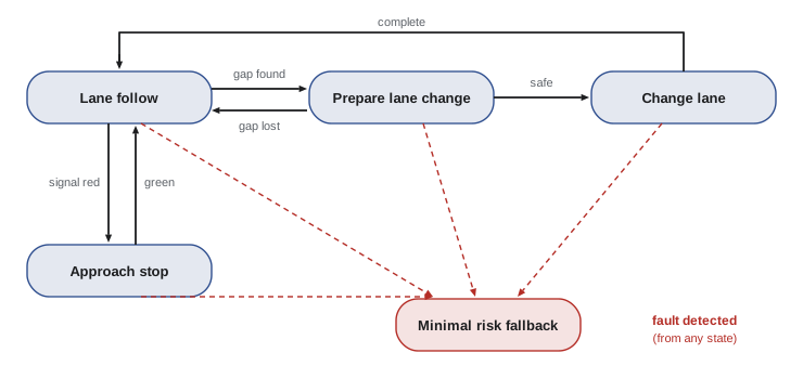
The behavior planner chooses the high-level maneuver: follow the lane, change lanes left or right, prepare to turn, stop at the line, yield to a pedestrian, pull over. Its output constrains the motion planner of Lesson 5, which computes the exact trajectory. Classic designs use finite-state machines: states such as lane follow, prepare lane change, change lane and stop, with transitions guarded by conditions like gap available or signal red. State machines are transparent and easy to test, but the number of states and transitions explodes as the operational design domain grows, and edge cases fall between rules.
Other designs score candidate behaviors with a cost function that weighs safety, progress, comfort and rule compliance, choosing the lowest-cost option. Hierarchical behavior trees, borrowed from robotics and games, organize decisions into reusable subtrees. Probabilistic approaches such as partially observable Markov decision processes, POMDPs, explicitly reason about uncertain intent: is that car going to turn, and how will the answer change as I learn more? They are principled but computationally heavy, so practical systems approximate them.
Rule-based versus learned decision-making
A major architectural debate concerns how much of the decision-making should be learned. At one end, modular stacks with hand-engineered rules make each decision traceable to a requirement, which suits safety cases and regulation. At the other, end-to-end systems train a single network from sensor input to trajectory, learning from large quantities of human driving and simulation. Proponents argue end-to-end learning scales better to the long tail of situations that rules never anticipate; critics point out that such systems are harder to verify, may copy human errors and can fail unpredictably outside their training distribution.
Most deployed systems at the time of writing (October 2026) blend the two. Learned components handle perception and prediction and propose candidate trajectories, while rule-based layers enforce hard constraints: never enter an occupied crosswalk, never exceed the speed limit by more than a set margin, always keep a safe following distance. These guardrails can be checked independently, an idea related to the responsibility-sensitive safety model discussed in Lesson 5. Whatever the architecture, the system must be able to explain, at least after the fact, why it did what it did, so that incidents can be investigated.
Worked problem
Cost-based choice between behaviors
A behavior planner scores three options with cost = 10 x risk + 1 x delay (s) + 2 x discomfort. Keep lane behind a slow truck: risk 0.01, delay 20 s, discomfort 0. Change lane left: risk 0.05, delay 2 s, discomfort 1. Hard brake and wait for a gap: risk 0.02, delay 8 s, discomfort 3. Which does it choose?
Show solution
- Keep lane: \( 0.1 + 20 + 0 = 20.1 \).
- Change lane: \( 0.5 + 2 + 2 = 4.5 \).
- Brake and wait: \( 0.2 + 8 + 6 = 14.2 \).
Answer: Change lane, cost 4.5. Note how the result depends entirely on the weights: with a risk weight of 400 instead of 10, keeping the lane would win, which is why weight choices must be justified and tested.
Common mistakes
MistakeAveraging multimodal predictions into one path.
InsteadKeep distinct hypotheses with probabilities; an average may be a path nobody takes.
MistakePlanning against only the most likely prediction.
InsteadCheck safety against all plausible futures, weighted by probability and severity.
MistakeTreating other road users as unaffected by the vehicle.
InsteadModel interaction; others react to what the automated vehicle does.
MistakeAssuming more caution is always safer.
InsteadFreezing and unpredictable hesitation create their own risks; be legible.
MistakeLetting a learned planner act without guardrails.
InsteadEnforce hard safety constraints that can be checked independently.
Summary and key terms
- Prediction estimates where other road users will go over the next several seconds.
- Futures are multimodal, so good predictors output several trajectories with probabilities.
- Physics models work for short horizons; map-aware and learned models capture intent.
- Interaction matters: others respond to the vehicle, and game-theoretic ideas help avoid collisions and deadlock.
- Behavior planning chooses maneuvers using state machines, cost functions, behavior trees or POMDP approximations.
- Deployed systems blend learned proposals with rule-based safety guardrails.
- Multimodal prediction
- Prediction that represents several distinct possible futures with probabilities.
- CTRV
- Constant turn rate and velocity motion model.
- minADE
- Minimum average displacement error over the top k predicted trajectories.
- Miss rate
- Fraction of cases where no prediction is close enough to the true future.
- Behavior planner
- The layer that selects high-level maneuvers such as lane changes or yielding.
- Finite-state machine
- A model with discrete states and guarded transitions.
- POMDP
- Partially observable Markov decision process, a framework for deciding under hidden state.
- Frozen robot problem
- Excessive caution that leaves a robot unable to act in dense traffic.
- Legibility
- Behaving so that others can readily infer your intent.
- End-to-end driving
- Training one model to map sensor input directly to driving output.
Practice problems
Work each problem on paper first, then reveal the answer to check.
Why is averaging two predicted paths dangerous?
Show answer
The average may be a path no agent would take, such as between lanes.
Typical prediction horizon for driving?
Show answer
About 3 to 8 seconds.
For how long does constant velocity work reasonably?
Show answer
About 1 to 2 seconds.
What does minADE measure?
Show answer
The smallest average error among the top k predicted trajectories.
Name a behavior planner design other than a state machine.
Show answer
Cost-based scoring, behavior trees or POMDP approximations.
What is the frozen robot problem?
Show answer
Being so cautious that the robot never finds a gap and blocks traffic.
How can a vehicle signal intent at a merge?
Show answer
Creeping forward, smooth acceleration or clear slowing.
What is conditional prediction?
Show answer
Predicting how others would respond to a specific action by the vehicle.
Why add rule-based guardrails to learned planners?
Show answer
They give checkable hard constraints for safety.
In the cost example, what risk weight makes keeping lane cheapest?
Show answer
Around 400 or higher.
Lesson quiz · 5 questions
Score 60% or more to complete this lesson.
Create a free account to save your progress, take quizzes and earn a certificate.