
ROB-320 · Lesson 2 of 12 · 30 min
Timing, measurement and worst-case execution time
A timing requirement is only as good as the numbers used to check it. This lesson is about getting those numbers: how long code takes to run, how much that varies, and what the longest possible time is. The longest time is called the worst-case execution time, or WCET, and it is the single most important number in real-time analysis, because every schedulability test in lesson 5 starts from it. Getting it wrong in the optimistic direction means a system that passes every analysis and still misses deadlines in the field. Getting it badly wrong in the pessimistic direction means buying a processor three times larger than needed.
Execution time is not a fixed property of a piece of code. It depends on the input data, which branches are taken, the state of the caches and pipelines when the code starts, what other cores are doing to shared memory and buses, and whether interrupts arrive mid-way. A measurement taken on a quiet bench with warm caches is a best case, not a worst case. The skill is to measure under conditions that push execution time up and to understand which effects the measurement may have missed.
Three ways to bound execution time
There are three broad approaches, and serious projects often use more than one.
- Measurement-based: run the code many times under stress and record the maximum. This is cheap and realistic, but it only finds the worst case that happened to occur. Engineers add a safety factor, often 20 to 50 %, to cover cases not exercised.
- Static analysis: tools model the processor's pipeline and caches and analyze every path through the compiled code to compute a guaranteed upper bound. This gives a safe number, but it needs a detailed processor model, struggles with complex multicore chips, and can be pessimistic. It is common in aerospace and automotive certification.
- Hybrid: measure execution times of small code segments on the target, then combine them along the worst path found by analyzing the program structure. This reduces pessimism while keeping some of the safety of analysis.
Whatever the method, the result should be written down with its conditions: compiler version and optimization level, clock frequency, cache configuration, and the load present during measurement. A WCET without conditions cannot be reused when anything changes.
Measuring with a GPIO pin and an oscilloscope
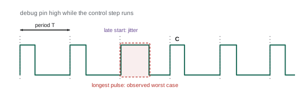
The simplest and most trustworthy measurement uses a spare output pin. Set the pin high at the start of the code under test and low at the end, then watch it on an oscilloscope or logic analyzer. The pulse width is the execution time, the spacing between pulses is the actual period, and the oscilloscope's persistence or histogram mode accumulates thousands of cycles so that the longest pulse and the widest spacing stand out. Toggling a pin costs only a few processor cycles, so it disturbs the timing very little, and the measurement is made by independent hardware rather than by the software being measured.
/* Bracket the control step with a GPIO pin for oscilloscope timing */
void control_isr(void)
{
    GPIOB->BSRR = PIN_DEBUG;          /* pin high: start of step  */
    read_encoder();
    compute_control();
    write_pwm();
    GPIOB->BSRR = PIN_DEBUG << 16;    /* pin low: end of step     */
}
Two refinements help. Use separate pins for different tasks so their interaction is visible, for example a pin that goes high whenever an interrupt is running. And measure from the hardware event rather than from the start of the code: triggering the oscilloscope on the timer or sensor signal and measuring to the end of the output write captures the interrupt latency and wake-up time too, which is the latency the controller actually experiences.
Cycle counters and software timestamps
Most modern processors include a free-running cycle counter. On ARM Cortex-M3 and higher cores it is the DWT CYCCNT register in the debug unit; on x86 it is the time-stamp counter read by RDTSC; RISC-V defines a cycle CSR. Reading the counter before and after a block and subtracting gives its execution time in cycles, which divided by the clock frequency gives seconds. Software timestamps make it easy to collect statistics over millions of runs and to store a histogram on the target, but the measurement itself takes time and the code that records it can disturb caches. Keep the bookkeeping tiny: update a running maximum and a histogram bin, and send the results out slowly from a low-priority task.
/* Cortex-M: measure a function with the DWT cycle counter */
CoreDebug->DEMCR |= CoreDebug_DEMCR_TRCENA_Msk;   /* enable trace unit   */
DWT->CYCCNT = 0;
DWT->CTRL  |= DWT_CTRL_CYCCNTENA_Msk;             /* start counting      */

uint32_t t0 = DWT->CYCCNT;
compute_control();
uint32_t cycles = DWT->CYCCNT - t0;               /* wrap-safe subtract  */
if (cycles > max_cycles) max_cycles = cycles;      /* running maximum     */
hist[cycles >> 6]++;                               /* 64-cycle bins       */
Worked problem
Converting cycles to time
A controller step on a 480 MHz processor takes between 31,200 and 58,700 cycles over a million runs. What are the best and worst observed execution times, and what WCET would you budget with a 30 % margin?
Show solution
- Best: \( 31{,}200 / 480 \times 10^{6} = 65 \) µs.
- Worst observed: \( 58{,}700 / 480 \times 10^{6} = 122.3 \) µs.
- Budgeted WCET: \( 122.3 \times 1.3 = 159 \) µs.
Answer: Observed times range from 65 to 122 µs; budget about 160 µs. The nearly two-to-one spread is typical of code that misses in cache or takes different branches on different cycles.
Why execution time varies
Understanding the sources of variation helps an engineer design measurements that find the true worst case.
| Source | Effect | How to provoke it in testing |
|---|---|---|
| Input-dependent branches | Different paths take different times | Drive inputs to limits, saturation and error cases |
| Caches | First access after eviction is much slower | Run cache-thrashing tasks or flush caches before each run |
| Shared buses and memory on multicore chips | Other cores delay memory access | Run memory-heavy load on all other cores |
| Interrupts and preemption | Higher-priority work stretches elapsed time | Generate maximum interrupt and network traffic |
| Frequency scaling and thermal throttling | Clock slows under heat or power limits | Pin frequency, test in a warm enclosure |
| Floating-point special cases | Denormal numbers can be very slow on some cores | Feed tiny values; enable flush-to-zero |
| Memory allocation and system calls | Unbounded or variable time | Remove from the control path entirely |
A useful distinction is between execution time, the processor time a job needs if it runs alone, and response time, the elapsed time from release to completion including time spent waiting for or preempted by other work. WCET is about the first; lesson 5 builds response time from it. Measurements made with a debug pin around the whole task capture response time unless interrupts are disabled, so label measurements carefully.
Worked problem
Multicore interference
A trajectory task runs in 180 µs worst case when the other three cores are idle. With a memory-heavy perception workload on the other cores, its worst case rises to 290 µs. What interference factor should the budget use, and why does it matter?
Show solution
- Factor: \( 290 / 180 = 1.61 \).
- The task's utilization at 1 kHz rises from 0.18 to 0.29.
Answer: Budget with the loaded value, an interference factor of about 1.6. On multicore systems-on-chip, shared caches and memory controllers make one core's timing depend on the others, so WCET must be measured with realistic load on every core, or the cores must be partitioned with cache and memory bandwidth controls.
Statistics of execution time
Execution-time distributions are not normal. They usually have a sharp lower edge, a main hump and a long thin tail to the right, where the rare slow cases live. The mean and standard deviation say almost nothing about the tail, and the tail is what causes deadline misses. Report the maximum, high percentiles such as the 99.9th and 99.999th, and a histogram on a logarithmic count axis that makes the tail visible. The number of runs matters: a one-in-a-million slow path will not appear in a ten-thousand-run test. For a 1 kHz loop, one hour of operation is 3.6 million cycles, so a soak test of several hours is a minimum for a hard real-time task.
import random
random.seed(7)
# Synthetic execution times (us): a main hump plus a rare slow path
samples = []
for i in range(2_000_000):
    t = 60 + random.gammavariate(4, 3)           # typical path
    if random.random() < 2e-5:                    # rare cache-cold case
        t += random.uniform(40, 70)
    samples.append(t)
first = max(samples[:10000])
samples.sort()
n = len(samples)
def pct(p):
    return samples[min(n - 1, int(p / 100 * n))]
mean = sum(samples) / n
print("mean     %.1f us" % mean)
for p in (50, 99, 99.9, 99.999):
    print("p%-7s %.1f us" % (p, pct(p)))
print("max      %.1f us" % samples[-1])
print("first 10,000 samples only, max %.1f us" % first)mean 72.0 us p50 71.0 us p99 90.2 us p99.9 99.3 us p99.999 126.1 us max 146.4 us first 10,000 samples only, max 110.7 us
The mean is 72 µs and the 99th percentile is 90 µs, but the maximum over two million runs is 146 µs, twice the mean. A ten-thousand-sample test tops out at about 111 µs: it sees the long tail of the normal path but none of the rare cache-cold cases. This is why a short bench test that 'never goes above 90 µs' is not evidence of a 90 µs WCET.
Tracing tools
Pins and counters time one thing at a time. Tracing tools record a timeline of everything: every task switch, interrupt entry and exit, lock acquisition and user-defined event, each with a timestamp. Hardware trace units such as ARM's Embedded Trace Macrocell stream instruction-level trace off the chip with almost no overhead. Software tracers built into operating systems record events into a memory buffer: FreeRTOS has trace hooks used by commercial and open-source viewers, Zephyr has a tracing subsystem, and Linux has ftrace, perf and the LTTng toolkit, with kernelshark and Trace Compass to view the results. ROS 2 has ros2_tracing, built on LTTng, which records callback start and end times so that end-to-end latency through a chain of nodes can be reconstructed.
A trace answers questions a single number cannot: which interrupt delayed the control task, which lower-priority task held a mutex, whether a periodic task drifted. The cost is data volume and some overhead, so traces are usually captured for short windows triggered by an anomaly, for example 'record continuously in a ring buffer and freeze it when the control task overruns'.
Worked problem
Sizing a trace buffer
An RTOS trace records 16-byte events. The system generates about 25,000 events per second. How much memory holds the last 2 seconds before a fault?
Show solution
- Events: \( 25{,}000 \times 2 = 50{,}000 \).
- Bytes: \( 50{,}000 \times 16 = 800{,}000 \) bytes, about 781 KiB.
Answer: About 800 kB, too much for many microcontrollers. Recording only scheduler and interrupt events, or storing 8-byte compressed events, brings it within reach; alternatively stream the trace off-chip through a debug probe.
Measuring periods and jitter
Execution time is half the story; the other half is whether tasks start when they should. Measure the actual period by timestamping each release and taking differences. Release jitter is the spread of start times relative to the ideal schedule, usually reported as the maximum deviation or as the difference between the largest and smallest observed periods. A periodic task should be released by a hardware timer, not by a software loop that sleeps for a fixed time after finishing its work, because sleeping a fixed time after variable work makes the period drift by the execution-time variation every cycle. Lesson 4 shows the correct RTOS call for absolute-time periodic waits, and lesson 9 shows the Linux equivalent.
On Linux, the standard tool for measuring how late the system wakes a high-priority thread is cyclictest from the rt-tests package. It runs threads that sleep until absolute times and records how late they actually wake. Lesson 9 uses its histograms to compare a standard kernel with a real-time one.
Common mistakes
MistakeTiming code on an idle bench with warm caches
InsteadMeasure under maximum realistic load with caches and buses contended.
MistakeReporting mean and standard deviation of execution time
InsteadReport maximum, high percentiles and a log-scale histogram.
MistakeRunning a short test and calling its maximum the WCET
InsteadSoak for millions of cycles and add a documented margin.
MistakeReleasing a periodic task with a relative sleep after the work
InsteadRelease it from a hardware timer or an absolute-time wait.
MistakeConfusing execution time with response time
InsteadLabel measurements and use WCET as the input to response-time analysis.
Summary and key terms
- Worst-case execution time is the key input to real-time analysis and depends on data, caches, buses and interrupts.
- WCET can be bounded by measurement with a margin, by static analysis, or by hybrid methods.
- A debug pin and an oscilloscope measure execution time, period and jitter with minimal disturbance.
- Cycle counters give software timestamps for statistics over millions of runs.
- Execution-time distributions have long right tails, so maxima and high percentiles matter, not means.
- Multicore interference can stretch execution time and must be measured with realistic load on all cores.
- Tracers record timelines of task switches and interrupts and explain why deadlines were missed.
- WCET
- Worst-case execution time: the longest time a piece of code can take to run in isolation.
- BCET
- Best-case execution time: the shortest time the code can take.
- Response time
- Elapsed time from a job's release to its completion, including waiting and preemption.
- Static timing analysis
- Computing a guaranteed WCET bound from the program and a processor model.
- Cycle counter
- A hardware register that counts processor clock cycles.
- Debug pin
- A spare output toggled by software so external instruments can time it.
- Release jitter
- Variation in when a periodic job actually starts.
- Interference
- Delay caused by other tasks, interrupts or cores sharing resources.
- Trace
- A timestamped record of system events such as task switches and interrupts.
- cyclictest
- A Linux tool that measures how late high-priority threads wake from timed sleeps.
Practice problems
Work each problem on paper first, then reveal the answer to check.
A step takes 96,000 cycles at 400 MHz. How long is that?
Show answer
240 µs.
Name the Cortex-M register used for cycle counting.
Show answer
DWT CYCCNT.
Why does a debug pin barely disturb timing?
Show answer
Toggling it costs only a few cycles and an external instrument does the measuring.
How many cycles does a 1 kHz loop run in 8 hours?
Show answer
28.8 million.
What is the difference between WCET and response time?
Show answer
WCET is isolated execution; response time includes waiting and preemption.
Give one way to provoke cache-related worst cases.
Show answer
Run cache-thrashing load or flush caches before each run.
A measured maximum is 75 µs. What WCET would a 40 % margin give?
Show answer
105 µs.
Why is the mean misleading for real-time work?
Show answer
It ignores the rare slow tail that causes misses.
What Linux tool reconstructs ROS 2 callback latency?
Show answer
ros2_tracing, built on LTTng.
Why should periodic tasks not use a relative sleep after their work?
Show answer
The period drifts by the variation in execution time.
Lesson quiz · 5 questions
Score 60% or more to complete this lesson.
Create a free account to save your progress, take quizzes and earn a certificate.