
ROB-320 · Lesson 1 of 12 · 31 min
Real-time requirements and latency budgets
A robot is a computer that has to keep appointments. Its current loop must run every 50 microseconds, its joint controller every millisecond, its safety monitor within a few milliseconds of any fault, and its planner fast enough that the robot does not stall waiting for a decision. Being right is not enough: a torque command that arrives 3 ms late can be as harmful as a wrong one, because the joint has already moved on. Real-time computing is the discipline of building software whose timing is as dependable as its arithmetic. This course follows on from ROB-200, which covered microcontrollers, peripherals and buses, and ROB-300, which designed controllers on paper and in simulation. Here the question is how those controllers actually run on processors that are also handling sensors, networks, logging and user interfaces, and how an engineer can show, rather than hope, that every deadline will be met.
This first lesson sets out the vocabulary: what makes a system real-time, the difference between hard, firm and soft deadlines, what latency and jitter mean in a control loop, and how to turn a controller's requirements into a timing budget that can later be checked task by task.
What real-time means
A real-time system is one whose correctness depends on when results are produced as well as on what they are. The common misconception is that real-time means fast. A system that answers in 10 microseconds most of the time but occasionally takes 30 milliseconds is fast on average and useless for control. A system that always answers within 2 milliseconds may be slower on average but is predictable, and predictability is what real-time engineering buys. The key property is a bounded worst case: for each job the system must do, there is a known upper limit on how long it can take, and that limit is below the deadline.
Three terms recur. A task is a unit of work the system performs repeatedly, such as reading an encoder and computing a torque. Each execution of a task is a job. A deadline is the time by which a job must finish, usually measured from its release, the moment it becomes ready to run. For periodic tasks the deadline is often equal to the period: the joint loop released every 1 ms must finish before the next release. Sporadic tasks, such as handling an emergency-stop input, have a minimum time between releases and a deadline measured from each event.
Hard, firm and soft deadlines
Deadlines differ in what happens when they are missed. The classic way to show this is with a value function: the usefulness of a result as a function of when it arrives.
- Hard: a missed deadline is a failure with potentially serious consequences. The value drops to zero or below at the deadline. Examples are the current loop of a motor drive, which must update the PWM duty cycle every switching period, and a safety function that must remove power within a specified stopping time.
- Firm: a late result is worthless but not harmful; the job is simply discarded. A camera frame that arrives after the next frame has already been captured is firm: a visual servoing loop uses the newest frame and drops the stale one.
- Soft: a late result is still useful but less so, and occasional misses degrade quality rather than causing failure. Logging, telemetry to an operator screen and path replanning are typically soft.
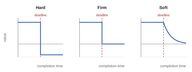
Most robots mix all three. The art is to identify which functions are hard, keep them small and isolated, and give them guaranteed resources, while letting soft functions share whatever capacity remains. A common mistake is to treat everything as hard, which makes the system expensive and hard to analyze, or to treat everything as soft, which works in the lab until a busy moment makes the control loop late.
Latency, jitter and why they matter to a controller
Latency is the delay from a cause to its effect: from the instant a sensor samples a joint position to the instant the drive applies the torque computed from it. Jitter is the variation in timing from one cycle to the next, either in when a task starts (release jitter) or in how long the whole sense-compute-act chain takes (latency jitter). Both matter to control. ROB-230 showed that a pure delay \( T_d \) adds a phase lag of \( \omega T_d \) radians at frequency \( \omega \), eating into phase margin. A loop with a crossover of 50 Hz and 2 ms of delay loses
of phase margin, which can turn a well-damped loop into an oscillating one. Jitter is worse than a constant delay because the controller cannot compensate for it: a fixed 1 ms delay can be modeled and designed around, but a delay that varies between 0.2 and 1.8 ms injects noise into the effective sample time, and discrete-time controllers designed for a fixed period behave as if their gains were changing every cycle.
Worked problem
Phase margin lost to delay
A velocity loop is designed with a crossover of 80 Hz and 55° of phase margin, assuming no computational delay. Measured sense-to-actuate latency is 0.75 ms. What phase margin remains?
Show solution
- Phase lost: \( 360^{\circ} \times 80 \times 0.00075 = 21.6^{\circ} \).
- Remaining margin: \( 55^{\circ} - 21.6^{\circ} = 33.4^{\circ} \).
Answer: About 33° remains, which typically shows as overshoot of roughly 35 % on a step. Either the latency must be cut, for example by moving the computation into the sensor interrupt, or the crossover lowered, or the delay included in the design model from the start.
Turning requirements into a latency budget
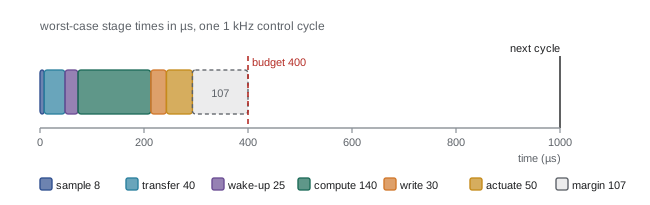
A latency budget divides the allowed end-to-end time among the stages a signal passes through, the same way a project budget divides money among tasks. For a joint position loop the chain usually looks like this: the encoder is sampled, its value is transferred over a bus, an interrupt or task wakes up, the controller computes, the result is written to the drive or PWM peripheral, and the drive applies it at its next update. Each stage has a typical and a worst-case time. The budget is met only if the sum of the worst cases, plus margin, fits inside the requirement.
| Stage | Typical (µs) | Worst case (µs) | Notes |
|---|---|---|---|
| Encoder sample and conversion | 5 | 8 | Fixed by sensor hardware |
| Bus transfer (SPI or EtherCAT) | 20 | 40 | Depends on frame size and bus load |
| Interrupt latency and task wake-up | 3 | 25 | Rises when other interrupts are active |
| Control computation | 60 | 140 | Branches, cache misses, floating point |
| Write to drive or PWM register | 10 | 30 | Shadow registers apply at next PWM edge |
| Drive update delay | 25 | 50 | Half a PWM period on average |
| Total | 123 | 293 | Budget: 400 µs, so worst-case margin is 107 µs |
Two habits make budgets useful. First, budget worst cases, not averages: a loop that meets its deadline on average misses it whenever several stages are slow at once. Second, keep explicit margin, commonly 20 to 30 % of the budget, because measured worst cases are only the worst seen so far, and software grows over a product's life. Later lessons show how to measure each stage (lesson 2), how to bound computation time on a processor shared with other tasks (lesson 5), and how interrupts and locks add to latency (lessons 6 and 7).
Worked problem
Checking a sensor-to-actuator budget
A gripper's force loop must respond within 2 ms. Worst-case stage times are: force sensor ADC 120 µs, I²C transfer 450 µs, task wake-up 80 µs, computation 300 µs, CAN message to the drive 260 µs, drive update 500 µs. Is there at least 20 % margin?
Show solution
- Sum of worst cases: \( 120 + 450 + 80 + 300 + 260 + 500 = 1710 \) µs.
- Margin: \( 2000 - 1710 = 290 \) µs, which is \( 290/2000 = 14.5\,\% \).
Answer: No: margin is only 14.5 %. The slow I²C link is the obvious target; moving the sensor to SPI (around 50 µs for the same data) would raise the margin to about 34 %.
Periods, rates and the control hierarchy
Robot software is usually layered by rate. Inner loops run fast and do little; outer loops run slowly and do a lot. A typical industrial arm runs current control at 10 to 20 kHz on the drive, velocity and position control at 1 to 8 kHz, trajectory interpolation at 1 kHz or so, collision checking and motion planning at tens of hertz, and perception at the camera frame rate. Each layer only needs to be a few times faster than the dynamics it controls and a few times slower than the layer inside it, which is why cascaded designs (ROB-300 lesson 11) map so naturally onto a set of periodic tasks.
The rate choice is a timing requirement in disguise. The rule of thumb from ROB-230 is to sample a loop at 10 to 30 times its closed-loop bandwidth. A position loop with 20 Hz bandwidth therefore wants at least 200 to 600 Hz, and choosing 1 kHz leaves room. Running faster than necessary is not free: every task's processor share is its execution time divided by its period, and lesson 5 shows that the total share decides whether the whole task set can meet its deadlines.
# Processor utilization of a robot task set: U = sum(C / T)
tasks = [  # name, worst-case execution time C (us), period T (us)
    ("current loop",   18,     50),
    ("joint loop",    140,   1000),
    ("trajectory",    220,   1000),
    ("safety monitor", 60,   2000),
    ("telemetry",     900,  20000),
    ("planner",      8000, 100000),
]
total = 0.0
for name, C, T in tasks:
    u = C / T
    total += u
    print("%-15s C=%5d us  T=%6d us  U=%.3f" % (name, C, T, u))
print("total utilization: %.3f (%.1f %% of one core)" % (total, 100 * total))current loop C= 18 us T= 50 us U=0.360 joint loop C= 140 us T= 1000 us U=0.140 trajectory C= 220 us T= 1000 us U=0.220 safety monitor C= 60 us T= 2000 us U=0.030 telemetry C= 900 us T= 20000 us U=0.045 planner C= 8000 us T=100000 us U=0.080 total utilization: 0.875 (87.5 % of one core)
The current loop, though tiny, is the largest single load because it runs 20,000 times a second. This is why current loops usually live in drive hardware or a dedicated microcontroller core rather than sharing a processor with planning.
Worked problem
Choosing a loop rate
A wheel velocity loop must reach a closed-loop bandwidth of 15 Hz. Its computation takes 45 µs. Pick a rate using the 10 to 30 times rule and give its processor share.
Show solution
- Rate range: \( 10 \times 15 = 150 \) Hz to \( 30 \times 15 = 450 \) Hz.
- Choose 500 Hz (period 2 ms) for a little extra margin and a round number.
- Share: \( 45/2000 = 0.0225 \), about 2.3 % of a core.
Answer: Run the loop at 500 Hz; it uses about 2.3 % of the processor. Going to 5 kHz would gain almost nothing in control quality and cost ten times the processor time.
Predictability over speed
Hardware and software features that make computers fast on average often make them less predictable. Caches speed up typical code but make execution time depend on what ran before. Branch predictors, speculative execution, dynamic voltage and frequency scaling, garbage-collected languages and virtual memory paging all trade worst-case behavior for average-case speed. Real-time designers do not always avoid these features, but they account for them: they measure under the worst realistic load, disable frequency scaling on control cores, lock critical code and data into memory, and keep hard real-time code in languages and runtimes with predictable timing, typically C, C++ or Rust without dynamic allocation in the control path.
The design principle that follows is separation. Put hard real-time functions on hardware and software that can be analyzed, keep their code small, and connect them to the large, fast-on-average parts of the system (Linux, perception, planning) through well-defined interfaces that cannot block the critical path. A robot arm whose safety stop depends on a Python process finishing garbage collection is badly designed however powerful its computer is.
A practical consequence shows up in procurement. When choosing a processor or board for a controller, the questions are not only clock speed and core count but whether the vendor documents interrupt latency, whether caches can be locked or partitioned, whether there is a tightly coupled memory region for critical code, whether frequency scaling can be pinned, and whether a real-time operating system or real-time Linux is supported. Many robot controllers pair a powerful application processor with a small microcontroller or real-time core on the same chip precisely so that the hard real-time work gets hardware with simple, documented timing.
Writing timing requirements well
A good timing requirement is specific and testable. 'The controller must be fast' is useless. 'The joint position loop shall execute every 1.000 ms ± 20 µs, and the time from encoder sample to PWM update shall not exceed 400 µs under maximum system load' can be designed for and verified. Good requirements state the period or minimum inter-arrival time, the deadline, the allowed jitter, the load conditions under which they apply and what the system must do if a deadline is missed: skip the cycle, hold the last output, raise a fault, or stop safely. This last point is often forgotten, yet it decides whether a rare overrun becomes a harmless glitch or a dangerous one.
Requirements should also say how timing will be verified. Measurement alone gives the worst case observed, not the true worst case; analysis gives bounds that may be pessimistic. Most robot projects combine the two: analysis to show the design can work, and long measurements under stress to show the implementation does. Lesson 2 begins with measurement.
Common mistakes
MistakeEquating real-time with high speed
InsteadDesign for a bounded worst case; predictability matters more than average speed.
MistakeBudgeting with typical or average stage times
InsteadAdd up worst-case times for every stage and keep explicit margin.
MistakeIgnoring jitter because the average period is right
InsteadBound and measure jitter, since controllers cannot compensate for varying delay.
MistakeTreating every function as hard real-time
InsteadClassify functions as hard, firm or soft and isolate the hard ones.
MistakeLeaving overrun behavior unspecified
InsteadState what the system does when a deadline is missed, such as holding output or stopping safely.
Summary and key terms
- A real-time system is correct only if its results arrive on time, so a bounded worst case matters more than average speed.
- Tasks release jobs periodically or sporadically, and each job has a deadline measured from its release.
- Hard deadlines must never be missed, firm results are useless when late, and soft results degrade gracefully.
- Latency adds phase lag of \( 360^{\circ} f_c T_d \) and jitter adds unpredictable variation that controllers cannot cancel.
- A latency budget sums worst-case stage times and keeps 20 to 30 % margin.
- Robot software is layered by rate, and each task's processor share is \( C/T \).
- Good timing requirements state period, deadline, jitter, load conditions, overrun behavior and verification method.
- Real-time system
- A system whose correctness depends on the timing of its results as well as their values.
- Task
- A unit of work executed repeatedly, such as one control loop.
- Job
- One execution of a task.
- Deadline
- The time by which a job must finish, measured from its release.
- Hard deadline
- A deadline whose miss counts as a system failure.
- Firm deadline
- A deadline after which the result is useless but causes no harm.
- Soft deadline
- A deadline whose miss reduces quality rather than causing failure.
- Latency
- The delay from a cause, such as a sensor sample, to its effect, such as an actuator update.
- Jitter
- Variation in timing from one cycle to the next.
- Latency budget
- An allocation of an end-to-end timing requirement across processing stages.
Practice problems
Work each problem on paper first, then reveal the answer to check.
Classify a motor drive current loop as hard, firm or soft.
Show answer
Hard.
Classify a live video preview on an operator tablet.
Show answer
Soft, or firm per frame.
How much phase is lost at 40 Hz with 1.5 ms delay?
Show answer
\( 360 \times 40 \times 0.0015 = 21.6^{\circ} \).
A task has C = 250 µs and T = 2 ms. What is its utilization?
Show answer
0.125.
Name two hardware features that improve average speed but hurt predictability.
Show answer
Caches and frequency scaling (also branch prediction, paging).
A budget has worst-case stages summing to 850 µs in a 1 ms cycle. What is the margin?
Show answer
150 µs, or 15 %.
Why is jitter harder to handle than a constant delay?
Show answer
A constant delay can be modeled and compensated; a varying one cannot.
What sample-rate range suits a loop with 25 Hz bandwidth?
Show answer
250 to 750 Hz.
What should a requirement say about missed deadlines?
Show answer
What the system does on an overrun, such as hold output or stop safely.
Why do current loops often run on drive hardware?
Show answer
Their high rate makes them the largest processor load and the tightest deadline.
Lesson quiz · 5 questions
Score 60% or more to complete this lesson.
Create a free account to save your progress, take quizzes and earn a certificate.