Sensor fusion in practice

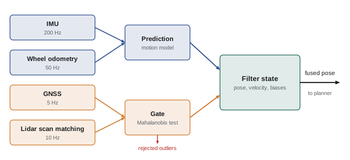
Real robots rarely rely on one sensor. A field robot might combine wheel encoders, an inertial measurement unit (IMU), a GNSS receiver and a lidar; an indoor robot, encoders, an IMU and scan matching against a map. Each sensor has different strengths, rates, latencies and failure modes, and a well-designed fusion filter lets each cover the others' weaknesses. The mathematics is the Kalman filter of lessons 5 to 7, but making it work on a real robot depends on a set of practical decisions that textbooks often skip: what goes in the state, how to handle measurements that arrive late or out of order, how to keep coordinate frames straight, and how to stop one bad measurement from corrupting everything. This lesson covers those decisions, with examples drawn from the common case of IMU, wheel odometry and GNSS fusion.

Complementary sensors

Sensors fall into two broad groups. Proprioceptive sensors, such as IMUs and wheel encoders, measure the robot's own motion. They are fast (often 100 to 1,000 Hz), smooth and always available, but they measure rates or increments, so integrating them accumulates error without bound: a gyro with a bias of 0.01°/s drifts 36° in an hour, and accelerometer bias integrated twice produces position error growing with the square of time. Exteroceptive sensors, such as GNSS, lidar and cameras, measure the robot's relation to the outside world. They give bounded, absolute information but are slower, noisier sample to sample, and subject to outages and outliers. Fusion exploits this complementarity: the proprioceptive sensors carry the estimate smoothly between exteroceptive updates, and the exteroceptive sensors stop the drift. ROB-220 introduced the complementary filter as a simple fixed-gain version of this idea; the Kalman filter does the same job with gains that adapt to the actual uncertainties.

Designing the state

The state must contain everything the motion and measurement models need, and it should include the hidden quantities that would otherwise violate the Markov assumption of lesson 2. For a ground robot fusing IMU, wheels and GNSS, a typical state is position, velocity and heading, often in three dimensions with roll and pitch, plus the gyro and accelerometer biases. Estimating biases is one of the most valuable things a fusion filter does: by comparing integrated gyro rate with heading changes implied by GNSS track or wheel odometry, the filter learns the gyro bias and removes it, so that during a GNSS outage the heading drifts far more slowly than with raw gyro integration. Bias states are modeled as random walks with small process noise, reflecting that biases change slowly with temperature and time.

There are two ways to use proprioceptive data. It can be treated as a control input in the prediction step, the usual choice for IMUs in inertial navigation, so the filter predicts at the IMU rate; or it can be treated as a measurement of velocity or angular rate, the usual choice for wheel odometry in packages such as robot_localization, where a kinematic model with velocity states is predicted at a fixed rate and odometry velocities update it. Using a sensor as a control means its noise must enter as process noise; using it as a measurement means its noise enters as measurement noise. Both are valid; mixing them carelessly, such as feeding the same wheel data as both a control and a measurement, double-counts information and makes the filter overconfident.

Time, latency and asynchronous measurements

Sensors run at different rates and their data arrive with different delays. A GNSS fix may describe where the robot was 100 ms ago; a lidar scan takes 100 ms to sweep, so its points were measured over a span of time; a camera image may arrive after 50 ms of processing. If the filter applies each measurement as though it describes the current moment, the errors are proportional to the robot's speed. Three practices handle this. First, timestamp every measurement at the moment it was taken, ideally in hardware or using a shared clock synchronized by the Precision Time Protocol (PTP) or a GNSS pulse-per-second signal, not when it arrives at the computer. Second, process measurements in timestamp order: the filter predicts forward to each measurement's time, applies the update, and continues. Third, for measurements that arrive late, after the filter has already moved past their timestamp, either keep a short history buffer and re-run the filter from the measurement's time (buffer and replay), or apply the update to a stored past state and propagate forward, or simply discard measurements that are too old.

Coordinate frames

Fusion bugs are often frame bugs. A ground robot typically uses the frames defined in ROS REP 105: base_link, fixed to the robot; odom, a world-fixed frame in which the pose is continuous and smooth but drifts over time; and map, a world-fixed frame in which the pose is globally accurate but may jump when a correction arrives. A common architecture runs one filter fusing only continuous sensors (wheels and IMU) to publish odom to base_link, and a second filter or a localization node adding GNSS or map-based corrections to publish map to odom. Controllers that need smooth local motion use the odom frame; planners that need global accuracy use the map frame. Each sensor also has its own mounting frame, and its measurements must be transformed using the measured position and orientation of the sensor on the robot. A GNSS antenna mounted 1 m behind the rear axle reports the antenna position, not the robot center; when the robot turns, the antenna moves sideways relative to the center, and ignoring this lever arm creates errors of tens of centimeters. For GNSS, latitude and longitude must also be converted to a local metric frame, such as east-north-up or UTM, as the navsat_transform node in robot_localization does.

Outlier rejection with Mahalanobis gating

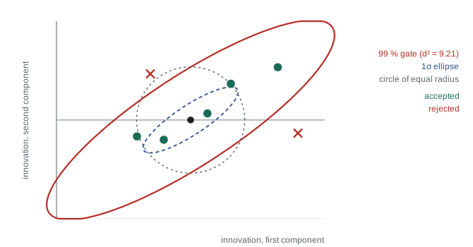
Exteroceptive sensors occasionally produce gross errors: GNSS multipath near buildings can jump by tens of meters, a scan matcher can lock onto the wrong wall, a wheel can spin on ice. A Kalman filter has no defense against these, because it trusts every measurement according to R. The standard defense is to check each measurement's innovation against its predicted covariance before using it. The squared Mahalanobis distance of the innovation is the NIS of lesson 5:

For a consistent filter, \( d^2 \) follows a chi-square distribution with as many degrees of freedom as the measurement has dimensions, so a threshold can be chosen for a desired false-rejection rate. For 99 % acceptance the thresholds are 6.63 for one dimension, 9.21 for two and 11.34 for three. Measurements beyond the gate are rejected or down-weighted. The gate must be used thoughtfully: if the filter has drifted badly during a long outage, good measurements may fall outside a gate computed from an overconfident covariance, and the filter will reject the very data that could save it. Implementations therefore track how many measurements in a row have been rejected and reset or widen the gate if the count grows, and they monitor the filter's covariance so that it reflects real uncertainty.

import numpy as np
def run(estimate_bias, seed=9):
    rng = np.random.default_rng(seed)
    dt, T = 0.01, 3000                                  # 100 Hz IMU, 30 s
    A = np.array([[1, dt, -dt*dt/2], [0, 1, -dt], [0, 0, 1]])   # state: position, velocity, accel bias
    B = np.array([dt*dt/2, dt, 0]); H = np.array([[1.0, 0, 0]]); R = 0.5**2
    qb = 1e-8 if estimate_bias else 0.0
    Q = np.diag([1e-8, 1e-4, qb]); S = np.diag([1.0, 1.0, 0.01 if estimate_bias else 0.0])
    x = np.array([0.0, 0.0, 0.05]); mu = np.zeros(3)    # true accel bias 0.05 m/s^2
    rejected, err = 0, []
    for k in range(T):
        a_true = 0.3*np.sin(0.2*k*dt)
        x[:2] = [x[0] + x[1]*dt + 0.5*a_true*dt*dt, x[1] + a_true*dt]
        a_meas = a_true + x[2] + rng.normal(0, 0.02)    # biased, noisy IMU
        mu = A @ mu + B*a_meas; S = A @ S @ A.T + Q
        if k % 20 == 0 and not (12 < k*dt < 22):        # GNSS at 5 Hz, outage from 12 s to 22 s
            z = x[0] + rng.normal(0, 0.5) + (15.0 if rng.random() < 0.05 else 0.0)   # 5 % multipath jumps
            y = z - mu[0]; s = S[0, 0] + R
            if y*y/s > 6.63: rejected += 1                # 99 % gate, 1 degree of freedom
            else:
                K = S @ H.T/s; mu = mu + K.ravel()*y; S = (np.eye(3) - K @ H) @ S
        err.append(abs(mu[0] - x[0]))
    err = np.array(err)
    print(f"bias state {'on ' if estimate_bias else 'off'}: estimated bias {mu[2]:.3f}, rejected fixes {rejected}, "
          f"median error {np.median(err):.2f} m, worst in outage {err[1200:2200].max():.2f} m")
run(True); run(False)

bias state on : estimated bias 0.042, rejected fixes 6, median error 0.24 m, worst in outage 1.16 m
bias state off: estimated bias 0.000, rejected fixes 6, median error 0.29 m, worst in outage 3.57 m

With the bias state, the filter learns most of the 0.05 m/s² accelerometer bias from the GNSS fixes before the outage (it estimates about 0.04), so during the ten seconds without GNSS the position error peaks at a little over a meter. Without the bias state, the same outage produces an error of about 3.6 m, close to the \( \tfrac{1}{2}bt^2 = 2.5 \) m of an uncorrected bias plus the velocity error it had already built up. In both runs the gate rejects the multipath jumps, each of which would otherwise yank the estimate by 15 m; removing the gate and re-running the simulation is an instructive exercise.

Off-the-shelf tools

Few teams write a fusion filter from scratch for a ground robot today. The robot_localization package for ROS 2 provides EKF and UKF nodes that fuse any number of odometry, IMU, pose and GNSS sources with per-sensor configuration of which variables to use, plus the navsat_transform node for GNSS. PX4 and ArduPilot autopilots include mature EKFs for drones, with innovation gating and sensor selection built in. Libraries such as GTSAM and Ceres support the smoothing approaches of lesson 10. Using these tools well still requires everything in this lesson: choosing which variables each sensor should update, setting covariances honestly, getting frames and timestamps right, and checking innovations to confirm the filter is consistent.