Sensor models

The correction step of the Bayes filter needs a measurement model, \( p(z_t \mid x_t) \): given that the robot is at state \( x_t \), how probable is the measurement it actually received? A good measurement model captures not only the sensor's random noise but also its failure modes: a lidar beam that passes through glass and returns the maximum range, a person who steps in front of the sensor, a reflection that produces a phantom wall. A model that knows only about Gaussian noise will be overwhelmed by these events; a model that expects them stays calm. This lesson develops the beam model and the likelihood field model for range sensors, the range-and-bearing model for landmarks, and the practical techniques that keep measurement updates robust.

What a measurement model must capture

Consider a single lidar beam pointed at a wall 4.0 m away. Most of the time it returns about 4.0 m, scattered by a centimeter or two of noise. Occasionally something unexpected, a person or a box not in the map, blocks the beam and it returns a shorter range. Sometimes the beam hits a black or shiny surface and no return is detected, so the sensor reports its maximum range. And now and then, for no identifiable reason, a reading is simply wrong. A measurement model that represents all of these is called a mixture model, because it mixes several simple distributions with weights that sum to 1. The weights and parameters are properties of the sensor and environment, and can be learned from logged data where the true pose is known.

The beam model

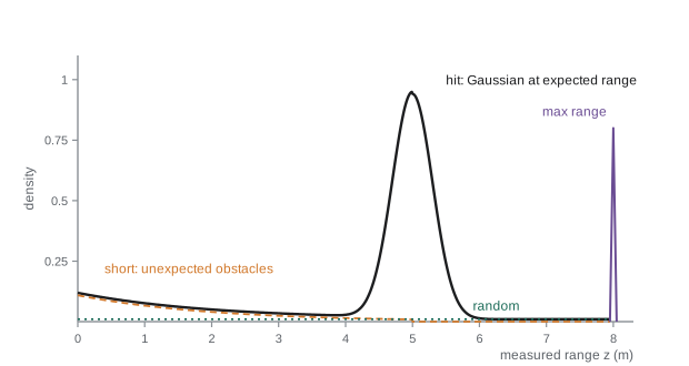
The beam model treats each range reading \( z^k \) in a scan independently given the pose. For a pose x and a map, the expected range \( z^{k*} \) is computed by ray casting: tracing the beam through the map until it hits an occupied cell. The likelihood of the actual reading is then a mixture of four parts:

\( p_{hit} \) is a Gaussian of standard deviation \( \sigma_{hit} \) centered on the expected range, truncated to the sensor's interval \( [0, z_{max}] \), representing correct readings with noise. \( p_{short} \) is an exponential distribution \( \lambda e^{-\lambda z} \) on \( [0, z^{k*}] \), representing unexpected objects, which are more likely to be detected close to the sensor because nearer objects block the beam first. \( p_{max} \) is a narrow spike at \( z_{max} \), representing missed returns. \( p_{rand} \) is uniform on \( [0, z_{max}] \), representing unexplained readings. The likelihood of the whole scan is the product over beams, \( p(z \mid x, m) = \prod_k p(z^k \mid x, m) \).

The likelihood field model

The beam model is physically motivated but has two drawbacks. Ray casting is expensive, since every beam must be traced through the map for every pose hypothesis, which matters for particle filters with thousands of particles and scans of hundreds of beams. And the beam model's likelihood can change abruptly with tiny pose changes: a beam that just grazes a table leg in one pose and misses it in another flips between very different expected ranges, making the likelihood surface jagged. The likelihood field model, also called the end-point model, avoids both. It projects the end point of each beam into the map from the hypothesized pose and asks only how far that end point is from the nearest obstacle:

where \( \text{dist}_k \) is the distance from the projected end point to the closest occupied cell. Beams reporting maximum range are usually discarded. The distances can be precomputed once for every cell of the map with a distance transform, so evaluating a scan costs one table lookup per beam instead of a ray cast. The likelihood surface is smooth, which helps both particle filters and optimization-based scan matching. The price is that the model ignores free space: a beam that passes straight through a mapped wall to an obstacle behind it is not penalized, because only its end point is checked. In practice the speed and smoothness outweigh this, and the likelihood field is the default in most localization packages.

Landmark measurement models

Many robots localize against distinct landmarks: reflectors, fiducial markers such as AprilTags, poles, or features extracted from images. A landmark sensor typically reports range r and bearing φ to landmark j at known position \( (m_{j,x}, m_{j,y}) \). The expected measurement from pose \( (x, y, \theta) \) is

and the measurement model adds Gaussian noise: \( r \sim \mathcal{N}(\hat{r}, \sigma_r^2) \), \( \phi \sim \mathcal{N}(\hat{\phi}, \sigma_\phi^2) \). Bearing differences must be wrapped into \( (-\pi, \pi] \), a source of countless bugs: a measured bearing of 179° and an expected bearing of −179° differ by 2°, not 358°. The Jacobian of this model with respect to the pose, needed by the extended Kalman filter, has a simple form with \( q = \hat{r}^2 \), \( \Delta x = m_{j,x} - x \) and \( \Delta y = m_{j,y} - y \):

A complication is data association: the sensor may see a landmark without knowing which one it is. Landmarks with unique identities, such as coded fiducial markers, avoid the problem; identical reflectors require matching each detection to a map landmark, covered in lesson 11.

Independence, correlated errors and robustness

Multiplying beam likelihoods assumes their errors are independent given the pose. Real scans violate this badly: neighboring beams hitting the same unmapped object, or a map that is slightly misaligned, produce errors that are strongly correlated. A filter that multiplies 1,000 correlated beams as if they were independent becomes wildly overconfident, collapsing its belief on the basis of what is really much less information. Three remedies are standard. Subsampling uses only every tenth or every thirtieth beam, which both speeds computation and reduces correlation. Inflating \( \sigma_{hit} \) beyond the sensor's true noise accounts for map errors and correlation; values of 10 to 20 cm are common for lidars whose datasheet noise is 1 to 3 cm. And tempering raises the scan likelihood to a power less than 1, such as \( p(z \mid x)^{1/10} \), which in log form simply divides the summed log-likelihood.

import numpy as np
rng = np.random.default_rng(11)
def beam_loglik(z, zstar, zmax=8.0, s=0.1, lam=0.5, w=(0.75, 0.1, 0.05, 0.1)):
    ph = np.exp(-0.5*((z - zstar)/s)**2)/(s*np.sqrt(2*np.pi))
    ps = np.where(z <= zstar, lam*np.exp(-lam*z)/(1 - np.exp(-lam*zstar)), 0.0)
    pm = (z >= zmax - 1e-9).astype(float)
    pr = np.full_like(z, 1/zmax)
    return np.log(w[0]*ph + w[1]*ps + w[2]*pm + w[3]*pr)
zstar = np.full(60, 5.0)                       # 60 beams, all expecting 5 m
z = zstar + rng.normal(0, 0.03, 60)            # a good scan
z_bad = z.copy(); z_bad[:6] = 2.0              # a person blocks 6 beams
z_off = zstar + 0.15 + rng.normal(0, 0.03, 60) # pose 15 cm wrong
for name, scan in [("good", z), ("6 blocked", z_bad), ("15 cm off", z_off)]:
    print(f"{name:10s} log-likelihood = {beam_loglik(scan, zstar).sum():8.1f}")
print("with tempering 1/10, good vs 15 cm off differ by",
      round((beam_loglik(z, zstar).sum() - beam_loglik(z_off, zstar).sum())/10, 1), "in log terms")

good       log-likelihood =     64.0
6 blocked  log-likelihood =     37.0
15 cm off  log-likelihood =     -7.2
with tempering 1/10, good vs 15 cm off differ by 7.1 in log terms

The six blocked beams cost the correct pose 27 units of log-likelihood (64.0 down to 37.0), because the short-reading component explains them as unexpected obstacles, so the correct pose still scores far above the misaligned one at −7.2. The raw difference of about 71 between the good pose and the 15 cm error corresponds to odds of \( e^{71} \approx 10^{31} \), far beyond anything justified when beam errors are correlated; tempering by a factor of 10 reduces the difference to 7.1, odds of about 1,200 to 1, which is still decisive but leaves room for other evidence. Choosing these robustness settings is part of tuning any localization system, and lesson 12 returns to it with a consistency test.