Particle filters and Monte Carlo localization

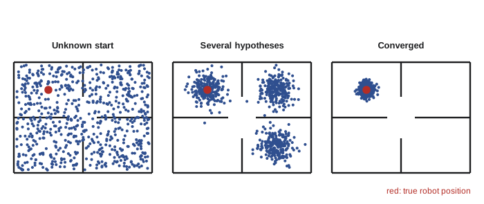
Gaussian filters summarize the belief with a mean and covariance, which fails when the belief has several peaks or a strongly curved shape. The particle filter makes no such assumption. It represents the belief by a large set of samples, called particles, each a complete guess of the state, and it implements the Bayes filter by moving the particles with the motion model, weighting them by the measurement model and resampling them so that likely hypotheses multiply and unlikely ones die out. With enough particles it can represent any distribution, including the multimodal beliefs of global localization. Applied to robot localization on a map, it is called Monte Carlo localization (MCL), introduced by Dellaert, Fox, Burgard and Thrun in 1999 and now the standard method for indoor mobile robots, including the AMCL package used throughout the ROS ecosystem. This lesson explains the algorithm, its key design choices and the failure modes to guard against.

Representing a belief with samples

A particle set \( \{(x^{[i]}, w^{[i]})\}_{i=1}^{N} \) represents a belief by N states with normalized weights. Probabilities of regions are approximated by the total weight of the particles inside them, and expectations by weighted sums, \( E[f(x)] \approx \sum_i w^{[i]}f(x^{[i]}) \). The approximation improves as N grows, with errors shrinking roughly in proportion to \( 1/\sqrt{N} \). Unlike a histogram, particles concentrate where the probability is, so they spend computation on the relevant parts of the state space; unlike a Gaussian, they can represent several hypotheses, banana shapes and hard boundaries such as walls the robot cannot be inside.

Importance sampling

The key idea behind the measurement update is importance sampling. Suppose we can draw samples from a proposal distribution q(x) but want them to represent a target distribution p(x). Weighting each sample by \( w = p(x)/q(x) \) corrects the mismatch: weighted averages over samples from q estimate expectations under p. In the particle filter, the proposal is the predicted belief, from which particles are drawn by sampling the motion model, and the target is the posterior, which by Bayes' rule is proportional to the predicted belief times the likelihood. The ratio is therefore simply the measurement likelihood:

This is what makes the particle filter so easy to implement: you only need to sample from the motion model (lesson 3) and evaluate the measurement likelihood (lesson 4). No Jacobians, no Gaussian assumptions.

The particle filter algorithm

The basic algorithm, called sampling importance resampling (SIR), repeats three steps each time a control and measurement arrive:

• Sample: for each particle, draw a new state from the motion model, \( x_t^{[i]} \sim p(x_t \mid x_{t-1}^{[i]}, u_t) \).
• Weight: compute \( w_t^{[i]} = p(z_t \mid x_t^{[i]}) \) for each particle, then normalize the weights to sum to 1.
• Resample: draw N new particles from the current set with replacement, each chosen with probability equal to its weight, and reset all weights to 1/N.

Resampling is the step that gives the particle filter its power and its pitfalls. It focuses computation on likely regions, since particles with high weight are duplicated and those with negligible weight disappear, so the next motion step spreads many particles around the good hypotheses. But it also discards information: every resampling step loses some diversity, and if the motion noise is small, duplicated particles stay clustered and the set can collapse onto a few states.

Resampling methods and effective sample size

Multinomial resampling, drawing N independent random numbers and picking particles by inverting the cumulative weight, works but adds unnecessary randomness. Systematic resampling, also called low-variance resampling, draws a single random number \( r \sim U[0, 1/N) \) and selects the particles at the points \( r, r + 1/N, r + 2/N, \ldots \) along the cumulative weights. It runs in linear time, preserves the set exactly when all weights are equal, and introduces much less sampling noise, so it is the standard choice.

Resampling every step is wasteful when the weights are nearly equal, because it only loses diversity. A common rule is to resample only when the weights have become uneven, measured by the effective sample size

which equals N when all weights are equal and 1 when one particle holds all the weight. Many implementations resample when \( N_{\text{eff}} \) falls below N/2. Between resamplings, weights are multiplied by each new likelihood and renormalized.

How many particles?

The number of particles needed depends on how spread out the belief is relative to how sharp the measurement likelihood is. Global localization in a large building may need tens of thousands of particles at first, because they must cover all free space densely enough that some land near the true pose; once the robot is localized, a few hundred suffice to track it. KLD-sampling (Fox, 2003) adapts N automatically: it bins the state space and keeps drawing particles until enough bins are occupied that the Kullback–Leibler divergence between the particle approximation and the true belief is likely below a bound. AMCL in ROS uses exactly this, with minimum and maximum particle counts as parameters. The fundamental limitation is dimension: covering a space densely needs a number of particles that grows exponentially with its dimension, so plain particle filters are practical for planar poses (three dimensions) and small extensions, not for the dozens of dimensions of a full SLAM state or a humanoid. Lesson 10 and ROB-340 show how Rao–Blackwellized particle filters and factor graphs get around this.

import numpy as np
rng = np.random.default_rng(4)
LM = np.array([[1.0, 9.0], [9.0, 9.0], [9.0, 1.0], [1.0, 1.0]])
def ranges(p): return np.hypot(LM[None, :, 0] - p[:, None, 0], LM[None, :, 1] - p[:, None, 1])
def systematic(w):
    N = len(w); pos = (rng.random() + np.arange(N))/N
    return np.minimum(np.searchsorted(np.cumsum(w), pos), N - 1)
N, sr = 3000, 0.15
true = np.array([[3.0, 4.0, 0.0]])
P = np.c_[rng.uniform(0, 10, N), rng.uniform(0, 10, N), rng.uniform(-np.pi, np.pi, N)]
w = np.full(N, 1/N)
for t in range(40):
    u = (0.2, 0.1)                                              # forward 0.2 m, turn 0.1 rad
    true[0, 2] += u[1]; true[0, :2] += u[0]*np.array([np.cos(true[0, 2]), np.sin(true[0, 2])])
    P[:, 2] += u[1] + rng.normal(0, 0.03, N)
    d = u[0] + rng.normal(0, 0.03, N); P[:, 0] += d*np.cos(P[:, 2]); P[:, 1] += d*np.sin(P[:, 2])
    z = ranges(true)[0] + rng.normal(0, sr, 4)
    w *= np.exp(-0.5*np.sum(((ranges(P) - z)/sr)**2, axis=1)); w /= w.sum()
    neff = 1/np.sum(w**2)
    if neff < N/2: P = P[systematic(w)] + rng.normal(0, 0.03, (N, 3)); w = np.full(N, 1/N)  # roughening
    if t + 1 in (1, 5, 10, 20, 40):
        e_xy = np.hypot(*(w @ P[:, :2] - true[0, :2]))
        th = np.arctan2(w @ np.sin(P[:, 2]), w @ np.cos(P[:, 2])); e_th = abs((th - true[0, 2] + np.pi) % (2*np.pi) - np.pi)
        print(f"step {t+1:2d}: N_eff {neff:7.1f}   position error {e_xy:.3f} m   heading error {np.degrees(e_th):6.1f} deg")

step  1: N_eff     5.6   position error 0.174 m   heading error  159.7 deg
step  5: N_eff   925.6   position error 0.160 m   heading error   32.6 deg
step 10: N_eff  2153.1   position error 0.207 m   heading error   17.6 deg
step 20: N_eff   939.2   position error 0.075 m   heading error    6.7 deg
step 40: N_eff  1793.2   position error 0.012 m   heading error    0.9 deg

Starting from 3,000 particles spread over the whole 10 m by 10 m area, the first measurement makes the weights extremely uneven: the effective sample size collapses to about 6, and the weighted position estimate is already within 20 cm. The heading is a different story. Range measurements say nothing directly about heading, so after one step the heading estimate is essentially random (160° off). Heading is recovered only gradually, because only particles with the right heading move in a way that keeps matching later measurements: 33° off after 5 steps, 7° after 20 and under 1° after 40, by which time the position error has fallen to about a centimeter. This is the filter extracting information from consistency over time. The small random jitter added after each resampling, called roughening, matters here: without it, the resampled particles cluster too tightly, no particle lies near the true heading, and the position error drifts while the filter waits for motion noise alone to explore.

Failure modes and remedies

Particle deprivation occurs when no particles remain near the true state, so the filter cannot recover even with perfect measurements. It happens after aggressive resampling with too few particles, too little motion noise, or an overconfident measurement model. Remedies include more particles, resampling only when \( N_{\text{eff}} \) is low, slightly inflated motion noise ('roughening') and tempered likelihoods. The kidnapped robot problem is the extreme case: someone picks the robot up and puts it elsewhere, or it slips badly on a ramp, and the particle set confidently tracks the wrong place. MCL detects this by watching the average measurement likelihood. Augmented MCL keeps two moving averages of it, a fast one \( w_{fast} \) and a slow one \( w_{slow} \), and injects random particles with probability \( \max(0, 1 - w_{fast}/w_{slow}) \): when recent measurements fit much worse than usual, a growing fraction of particles is scattered across the map, ready to catch the true pose. AMCL exposes these smoothing rates as parameters, usually named recovery_alpha_slow and recovery_alpha_fast.