Pumps and hydronic balancing

The secondary pumps at Riverbend were two 60 hp end-suction pumps on variable-frequency drives, one running and one standby. In August the operators noticed that the running pump's drive was at full speed most afternoons, even on moderate days, and the far building's coils were starved. Raj asked Theo to work out what the pump was actually doing. "You can't fix a hydronic system you haven't put on a curve," he said, handing him the pump's submittal and a differential pressure gauge.

Chillers and coils only work if the right amount of water reaches them. This lesson covers centrifugal pump curves and system curves, the affinity laws and variable-speed pumping, differential pressure control, balancing valves and how a system is balanced, and the corrections needed when the fluid is a glycol mixture instead of water.

Pump curves and system curves

A centrifugal pump adds pressure, usually called head, to the water it moves. Its performance curve, from the manufacturer's test, shows the head it produces at each flow at a given speed: high head at low flow, falling as flow increases. The curve sheet also shows the pump's efficiency, the power it needs, and its net positive suction head required at each flow, the minimum suction pressure to avoid cavitation. A pump should run near its best efficiency point, where the efficiency curve peaks.

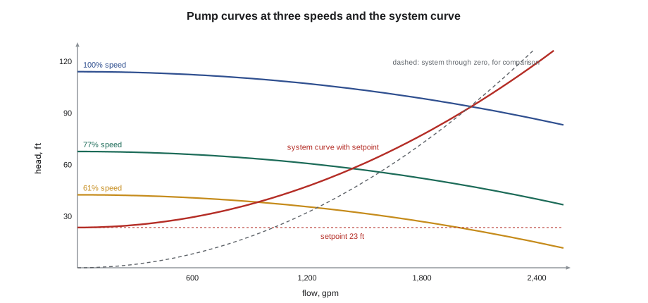
The piping system has a curve too. Pushing water through pipes, fittings, coils, valves and chillers takes pressure that rises with roughly the square of the flow. In a closed loop there is no static lift, because the water that goes up comes down again, so the system curve of a simple loop starts at zero head. A variable-flow loop controlled to hold a differential pressure at its far end has a system curve that starts at that setpoint, because the pumps must always provide it, and rises from there.

The pump runs where its curve crosses the system curve. To deliver a different flow, either the pump curve or the system curve must change: a throttling valve raises the system curve, wasting energy across the valve; a variable-speed drive lowers the pump curve, which is far more efficient.

The affinity laws

For a given pump and impeller, the affinity laws relate speed to flow, head and power: flow changes in proportion to speed, head with the square of speed, and power with the cube. Halving the speed of a pump on a system with no fixed head would cut its power to an eighth. This is why variable-speed pumping saves so much energy, and why the same laws apply to fans and, approximately, to centrifugal compressors.

In a real variable-flow system, though, the pump cannot follow the cube law all the way down, because the differential pressure setpoint holds part of the head constant. The savings are still large but smaller than the cube law suggests, which the script shows.

Putting Riverbend's secondary pump on a curve

Theo fitted the pump's full-speed curve from the submittal, estimated the system curve from the design flow and head and the 23 ft differential pressure setpoint at the far building, and found the speed and power at three flows: design, a typical afternoon, and a mild-weather night.

import math
H0, a = 114.0, 0.0000048                        # ft of head and ft/gpm^2
Hc, k = 23.4, 0.0000166                         # ft held at the far coil, and the piping and coil resistance
def operating(speed):
    q = math.sqrt((H0 * speed ** 2 - Hc) / (a + k))
    return q, Hc + k * q * q
full = None
for flow_target in (2045, 1430, 950):
    lo, hi = 0.3, 1.0
    for _ in range(60):
        mid = (lo + hi) / 2
        lo, hi = (mid, hi) if operating(mid)[0] < flow_target else (lo, mid)
    q, h = operating(hi)
    bhp = q * h / (3960 * 0.78)
    full = full or (q, bhp)
    print(f"flow {q:6,.0f} gpm at {h:5.1f} ft, speed {hi:.0%}, about {bhp:5.1f} bhp ({bhp * 0.746 / 0.93:.1f} kW input)")
print(f"the cube law alone would predict {full[1] * (950 / full[0]) ** 3:.1f} bhp at 950 gpm; the pressure setpoint keeps it higher")
# balancing valve: gpm = Cv x sqrt(dP in psi)
cv, dp_psi = 46.0, 1.8
print(f"balancing valve Cv {cv:.0f} at {dp_psi} psi: {cv * math.sqrt(dp_psi):.1f} gpm")
# brewery glycol loop: 35 % propylene glycol needs more flow than water for the same capacity
gpm_w = 2 * 12000 / (500 * 7.2)
factor = (1.0 * 1.0) / (0.90 * 1.03)            # specific heat 0.90 Btu/lb F and specific gravity 1.03 for the glycol
print(f"2 tons at 7.2 F: water {gpm_w:.2f} gpm, glycol {gpm_w * factor:.2f} gpm ({factor - 1:+.0%})")

flow  2,045 gpm at  92.8 ft, speed 100%, about  61.5 bhp (49.3 kW input)
flow  1,430 gpm at  57.3 ft, speed 77%, about  26.5 bhp (21.3 kW input)
flow    950 gpm at  38.4 ft, speed 61%, about  11.8 bhp (9.5 kW input)
the cube law alone would predict 6.2 bhp at 950 gpm; the pressure setpoint keeps it higher
balancing valve Cv 46 at 1.8 psi: 61.7 gpm
2 tons at 7.2 F: water 6.67 gpm, glycol 7.19 gpm (+8%)

At design flow, about 2,045 gpm, the pump ran at full speed and needed about 62 bhp. At 1,430 gpm it needed about 77 % speed and 27 bhp, and at 950 gpm about 61 % speed and under 12 bhp, but the pure cube law would have predicted about 6 bhp, because the pump still had to hold the setpoint at the far end.

So why was the real pump at full speed on moderate afternoons? The low delta-T from lesson 7 was part of it: the coils were drawing design flow at a fraction of design load. The other part was the setpoint. Someone had raised the differential pressure setpoint to 47 ft to fix the starved far building, which pushed the pump to full speed and still did not cure the starving, because the far building's balancing valves had been closed down during a renovation and never reopened. Raising the setpoint is a common fix for a distribution problem and almost always the wrong one.

Differential pressure control and reset

In a variable-flow system the pumps are usually controlled to hold the differential pressure across the supply and return at a sensor near the hydraulically most remote coil, the one that needs the most pump head to receive its flow. Placing the sensor at the pumps instead wastes energy, because the setpoint must then include the pipe losses at full flow even when the flow is low. Better still is setpoint reset: the controls lower the setpoint until at least one coil valve is nearly fully open, so the pumps provide just enough pressure for the most demanding coil at each moment. RAC-230 lesson 9 described the same idea for air systems.

The setpoint should be just enough for the most remote coil's valve, its piping branch and its balancing valve to pass design flow. At Riverbend, after the far building's valves were reopened and set, the setpoint was returned to 23 ft and a reset strategy added, which the controls contractor programd from the coil valve positions.

Balancing

Balancing divides the water among the coils in proportion to their design flows, so that the coils near the pumps, which see the most pressure, do not take more than their share and starve those far away. Constant-flow systems are balanced with manual balancing valves, which have a calibrated orifice or a valve body with pressure ports, so that the flow can be read with a differential pressure meter and the valve's flow coefficient, Kv in SI or Cv in US units.

The usual procedure, called proportional balancing, is the same as for air in RAC-330 lesson 8: measure every branch and coil, find the one with the lowest ratio of measured to design flow, and adjust the others in turn so that all have the same ratio, then raise the total flow until the reference coil reaches its design. Variable-flow systems with pressure-independent control valves need little or no manual balancing, because each valve limits its coil's flow to the set maximum whatever the pressure upstream. Many plants still have a mix of both, and a technician must know which kind of valve is on each coil before turning anything.

The script's balancing valve line converts a reading to flow. A valve with a Cv of 46 reading 1.8 psi passes about 62 gpm. On the far building's main branch, Theo found the valve at less than half its design flow, with its handle set two turns from closed, and a note on the drawing from the renovation contractor that it had been closed to fill and flush the new piping.

Cavitation, air and other pump troubles

Pumps fail in recognizable ways. Cavitation, caused by too little suction pressure, sounds like gravel in the pump and erodes the impeller; it is more common on open tower systems, where the pump draws from a basin, than on closed loops, which are pressurized. Air in a closed loop gathers at high points and in pump casings, reduces flow and makes noise; air separators and automatic vents remove it, and the expansion tank and makeup pressure must keep every high point above atmospheric pressure. Worn impellers and wear rings reduce a pump's head; a pump that cannot reach its curve at full speed may need an overhaul. Misalignment, worn couplings and bearing problems show up as vibration and heat, which a technician can check with the same tools as on any rotating machine.

Strainers protect pumps and coils from debris but block when full, raising the head the pump must provide; their pressure drop should be logged and they should be cleaned on a schedule, especially after work on the piping. Riverbend's renovation had left construction debris in the far building's strainers too.

Glycol corrections

Loops exposed to freezing, such as the brewery's process chiller, heat recovery loops with outdoor coils, and some tower free-cooling circuits, use a mixture of water and propylene or ethylene glycol. Glycol lowers the freezing point but changes the fluid's properties: its specific heat is lower than water's, its density slightly higher and its viscosity much higher, especially when cold. For the same capacity and delta-T, a glycol loop needs more flow; the higher flow and viscosity raise the pressure drop; and the coils and chillers transfer less heat, so their capacity must be corrected with the manufacturer's glycol factors.

The script's last part checks the brewery's 2-ton glycol chiller loop from RAC-110, which ran a 35 % propylene glycol mixture. For the same 7.2 °F delta-T, it needed about 8 % more flow than water. The pressure drop increase was larger, because of the viscosity, so the brewery's pump had been selected with that in mind. When topping up a glycol loop, technicians should add premixed fluid of the same type and concentration, not plain water, and check the concentration with a refractometer, because diluted glycol loses its freeze protection and its corrosion inhibitor.