Curved spacetime: metrics, geodesics and the geodesic equation

The equivalence principle told us that gravity is geometry: free bodies follow preferred worldlines that do not depend on what the bodies are made of, and over small regions spacetime looks flat. This lesson supplies the mathematics to make that idea precise. A curved spacetime is described by a metric, a rule that gives the interval between any two nearby events. Freely falling bodies follow geodesics of that metric, the worldlines of greatest proper time. The equation for geodesics involves the Christoffel symbols, which play the role of the gravitational field. By the end of the lesson we will have recovered Newton's law of gravity as the geodesic equation of a slightly warped time. MATH-430 developed geodesics on curved surfaces with a positive-definite metric; here the same machinery is applied to the four-dimensional spacetime of physics, with its minus sign.

The metric

On a flat plane in Cartesian coordinates the distance between nearby points is \(ds^2 = dx^2 + dy^2\). In polar coordinates the same plane has \(ds^2 = dr^2 + r^2 d\phi^2\). The coefficients look different, but the geometry is the same, because one set of coordinates can be transformed into the other. On a sphere of radius \(a\), with colatitude \(\theta\) and longitude \(\phi\), the distance is

and no change of coordinates can make this \(dx^2 + dy^2\) everywhere, because the sphere is intrinsically curved. In general, a metric in coordinates \(x^\mu\) is written

with a symmetric matrix of functions \(g_{\mu\nu}\). In four-dimensional spacetime there are ten independent components. The metric does three jobs at once. It gives the proper time along timelike worldlines, \(d\tau^2 = -ds^2/c^2\), and the proper length along spacelike curves. It determines which directions are timelike, null and spacelike at each point, so it fixes the light cones and with them the causal structure. And through its derivatives it determines how freely falling bodies move. The metric is the gravitational field.

At any single event it is always possible to choose coordinates in which \(g_{\mu\nu} = \eta_{\mu\nu}\) and the first derivatives of \(g_{\mu\nu}\) vanish. These are locally inertial coordinates, the mathematical form of a freely falling laboratory. The second derivatives cannot all be made to vanish; they contain the curvature, the part of gravity that the equivalence principle cannot remove. This is exactly parallel to a surface: at any point a small enough patch of the Earth looks flat, and a map can be drawn that is accurate to first order near that point, but no map of a large region keeps all distances correct.

Weak-field metric

The metric that describes the gravity of the Earth, the Sun and every slowly moving body in a weak field is, to good accuracy,

where \(\Phi\) is the Newtonian potential, \(-GM/r\) outside a spherical mass. The time part reproduces the gravitational time dilation of lesson 3: a clock at rest has \(d\tau = \sqrt{1 + 2\Phi/c^2}\,dt \approx (1 + \Phi/c^2)\,dt\). The space part says that rulers near the mass measure slightly more distance between given coordinate positions than they would far away: space is curved too. For slowly moving bodies only the time part matters. For light, which moves as fast in space as in time, both parts contribute equally, which is the origin of the factor of two in the bending of light.

Geodesics as worldlines of greatest proper time

In flat spacetime a free particle moves on a straight worldline, and lesson 2 showed that the straight timelike worldline between two events has the greatest proper time. In curved spacetime there are no straight lines, but there are worldlines of stationary proper time, and these are the geodesics. A freely falling particle moves between two events along the worldline that makes the proper time

stationary under small variations, where \(\lambda\) is any parameter along the path. This is a variational principle of exactly the type PHYS-344 studied. As there, it is easier to vary a simpler Lagrangian with the same extremals. Parametrizing by the proper time itself, the curves that extremize \(\tau\) also extremize

The Euler–Lagrange equation for coordinate \(x^\alpha\) is \(\frac{d}{d\tau}(\partial\mathcal{L}/\partial\dot{x}^\alpha) = \partial\mathcal{L}/\partial x^\alpha\). The left side gives \(\frac{d}{d\tau}(g_{\alpha\nu}\dot{x}^\nu) = g_{\alpha\nu}\ddot{x}^\nu + \partial_\mu g_{\alpha\nu}\,\dot{x}^\mu\dot{x}^\nu\), and the right side gives \(\frac{1}{2}\partial_\alpha g_{\mu\nu}\,\dot{x}^\mu\dot{x}^\nu\). Symmetrizing the middle term over \(\mu\) and \(\nu\) and multiplying by the inverse metric \(g^{\beta\alpha}\) gives the geodesic equation:

The \(\Gamma^\beta_{\mu\nu}\) are the Christoffel symbols. They are symmetric in their lower indices and built from first derivatives of the metric, so they vanish in locally inertial coordinates; this is the statement that a freely falling observer feels no gravitational force. They are not the components of a tensor, which is why they can be made to vanish at a point by a choice of coordinates. Written this way, the geodesic equation looks like Newton's second law with the Christoffel term as a force: the Christoffel symbols are the analog of the Newtonian gravitational field, and the metric is the analog of the potential. For light, which has no proper time, the same equation holds with \(\tau\) replaced by an affine parameter and with the extra condition \(g_{\mu\nu}\dot{x}^\mu\dot{x}^\nu = 0\).

Geodesics on a sphere

The sphere is the simplest curved space and a good place to practice. With \(ds^2 = a^2(d\theta^2 + \sin^2\theta\, d\phi^2)\), the only nonzero Christoffel symbols are

The geodesic equations are \(\ddot{\theta} - \sin\theta\cos\theta\,\dot{\phi}^2 = 0\) and \(\ddot{\phi} + 2\cot\theta\,\dot{\theta}\dot{\phi} = 0\). The second can be written \(\frac{d}{ds}(\sin^2\theta\,\dot{\phi}) = 0\), a conserved quantity that comes from the symmetry of the sphere under rotation about its axis, Clairaut's relation from MATH-430. The equator \(\theta = \pi/2\) with \(\dot{\phi}\) constant is clearly a solution; by symmetry, so is every great circle. Two geodesics that start parallel at the equator, both heading north, converge at the pole: positive curvature focuses geodesics. On a saddle-shaped surface of negative curvature, initially parallel geodesics diverge.

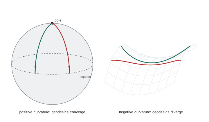
The code below computes the Christoffel symbols of a metric numerically, by finite differences of the metric components, and checks them against the formulas above. It then integrates the geodesic equation on a unit sphere starting from a point on the equator with a velocity tilted 40 degrees toward the north, and checks that the path stays on a great circle by measuring its distance from the plane through the sphere's midpoint that contains the starting point and direction.

import math
def christoffel(metric, x, h=1e-5):
    """Gamma^b_{mn} at point x for a metric function returning an n x n matrix."""
    n = len(x)
    g = metric(x)
    # inverse of a diagonal or 2x2 metric (enough for our examples)
    if n == 2:
        det = g[0][0]*g[1][1] - g[0][1]*g[1][0]
        gi = [[g[1][1]/det, -g[0][1]/det], [-g[1][0]/det, g[0][0]/det]]
    else:
        gi = [[(1/g[i][i] if i == j else 0.0) for j in range(n)] for i in range(n)]
    dg = []
    for k in range(n):                       # dg[k][a][b] = d g_ab / d x^k
        xp = list(x); xm = list(x); xp[k] += h; xm[k] -= h
        gp, gm = metric(xp), metric(xm)
        dg.append([[(gp[a][b] - gm[a][b]) / (2*h) for b in range(n)] for a in range(n)])
    G = [[[0.0]*n for _ in range(n)] for _ in range(n)]
    for b in range(n):
        for m in range(n):
            for nn in range(n):
                G[b][m][nn] = 0.5 * sum(gi[b][a] * (dg[m][a][nn] + dg[nn][a][m] - dg[a][m][nn]) for a in range(n))
    return G
sphere = lambda x: [[1.0, 0.0], [0.0, math.sin(x[0])**2]]       # unit sphere, x = (theta, phi)
th = 1.0
G = christoffel(sphere, [th, 0.3])
print("Gamma^theta_phiphi:", round(G[0][1][1], 6), " exact:", round(-math.sin(th)*math.cos(th), 6))
print("Gamma^phi_thetaphi:", round(G[1][0][1], 6), " exact:", round(1/math.tan(th), 6))
# integrate the geodesic equation with RK4 from the equator, heading 40 degrees north of east
def rhs(s):
    t, p, dt, dp = s
    return (dt, dp, math.sin(t)*math.cos(t)*dp**2, -2*dt*dp/math.tan(t))
def rk4(s, h):
    k1 = rhs(s); k2 = rhs([a + h/2*b for a, b in zip(s, k1)])
    k3 = rhs([a + h/2*b for a, b in zip(s, k2)]); k4 = rhs([a + h*b for a, b in zip(s, k3)])
    return [a + h/6*(b + 2*c + 2*d + e) for a, b, c, d, e in zip(s, k1, k2, k3, k4)]
ang = math.radians(40)
s = [math.pi/2, 0.0, -math.sin(ang), math.cos(ang)]    # theta decreases going north
xyz = lambda t, p: (math.sin(t)*math.cos(p), math.sin(t)*math.sin(p), math.cos(t))
r0, v0 = (1.0, 0.0, 0.0), (0.0, math.cos(ang), math.sin(ang))   # start point and direction
n = (r0[1]*v0[2] - r0[2]*v0[1], r0[2]*v0[0] - r0[0]*v0[2], r0[0]*v0[1] - r0[1]*v0[0])  # plane normal
worst, h, length, top = 0.0, 0.001, 0.0, 0.0
while length < 2.5:
    s = rk4(s, h); length += h
    p = xyz(s[0], s[1])
    worst = max(worst, abs(sum(a*b for a, b in zip(p, n))))
    top = max(top, 90 - math.degrees(s[0]))
print("arc length", round(length, 3), "rad; highest latitude reached", round(top, 2), "degrees (expected 40)")
print("largest distance from the great-circle plane:", f"{worst:.1e}")
print("Clairaut constant sin^2(theta) dphi/ds at the end:", round(math.sin(s[0])**2 * s[3], 6), " start:", round(math.cos(ang), 6))

Gamma^theta_phiphi: -0.454649  exact: -0.454649
Gamma^phi_thetaphi: 0.642093  exact: 0.642093
arc length 2.501 rad; highest latitude reached 40.0 degrees (expected 40)
largest distance from the great-circle plane: 2.1e-14
Clairaut constant sin^2(theta) dphi/ds at the end: 0.766044  start: 0.766044

Newton's law as a geodesic

Now apply the geodesic equation to the weak-field metric for a slowly moving particle. Slow means \(dx^i/d\tau \ll c\,dt/d\tau\), so in the sum \(\Gamma^i_{\mu\nu}\dot{x}^\mu\dot{x}^\nu\) the term with \(\mu = \nu = 0\) dominates, and \(d\tau \approx dt\). The geodesic equation for a spatial coordinate becomes

For a static metric \(\Gamma^i_{00} = -\frac{1}{2} g^{ij}\partial_j g_{00}\). With \(g_{00} = -(1 + 2\Phi/c^2)\) and \(g^{ij} \approx \delta^{ij}\) to first order, \(\Gamma^i_{00} = \partial_i \Phi/c^2\), so

which is Newton's law of gravitation. Only the time-time component of the metric entered. A slowly moving body falls because time runs at different rates at different heights, and the worldline of greatest proper time between two events bends toward the region where time runs slow. The spatial part of the metric, which is just as large, has no effect on slow bodies; it matters for light and for fast particles. This is why Newtonian gravity works so well for planets and why the bending of light came out wrong when Einstein had only the equivalence principle.

It is worth seeing the proper-time principle at work on a simple case. A ball is thrown straight up and caught one second later at the same spot. In a frame on the ground, its worldline rises and falls. Compare it with a ball that sits still for the same second. The thrown ball moves, so special-relativistic time dilation makes it age less; but it spends the second higher up, where clocks run faster, so gravity makes it age more. The real trajectory, rising to \(gT^2/8 = 1.2\) m and falling back, is precisely the one where the gain from height beats the loss from motion by the maximum amount. The code below checks this by computing the proper time along a family of trial worldlines with different peak heights.

c, g, T = 2.998e8, 9.81, 1.0
def proper_time_gain(hmax, n=4000):
    """Excess proper time (s) over a clock at rest, for a parabolic trial path peaking at hmax."""
    total = 0.0
    for i in range(n):
        t = (i + 0.5) * T / n
        z = 4 * hmax * t * (T - t) / T**2          # parabola through z = 0 at t = 0 and T
        v = 4 * hmax * (T - 2*t) / T**2
        total += (g * z / c**2 - v**2 / (2 * c**2)) * T / n   # weak-field d(tau)/dt - 1
    return total
best = max((proper_time_gain(h/100), h/100) for h in range(0, 301))
for h in (0.0, 0.5, 1.0, 1.226, 1.5, 2.5):
    print(f"peak {h:5.3f} m: extra proper time {proper_time_gain(h)*1e18:8.3f} attoseconds")
print("best peak height:", best[1], "m;  Newton predicts g T^2 / 8 =", round(g*T**2/8, 3), "m")

peak 0.000 m: extra proper time    0.000 attoseconds
peak 0.500 m: extra proper time   28.965 attoseconds
peak 1.000 m: extra proper time   43.094 attoseconds
peak 1.226 m: extra proper time   44.613 attoseconds
peak 1.500 m: extra proper time   42.390 attoseconds
peak 2.500 m: extra proper time   -3.523 attoseconds
best peak height: 1.23 m;  Newton predicts g T^2 / 8 = 1.226 m

The differences are only attoseconds, but the principle is exact. The peak that maximizes proper time is the Newtonian one to the resolution of the search. This is the deepest sense in which general relativity contains Newtonian gravity.

Covariant derivatives and parallel transport

The Christoffel symbols have a second meaning. In curved spacetime, comparing vectors at different points is not straightforward, because the coordinate basis vectors themselves change from point to point. The covariant derivative of a vector field, \(\nabla_\mu V^\nu = \partial_\mu V^\nu + \Gamma^\nu_{\mu\lambda} V^\lambda\), corrects the ordinary derivative for the turning of the basis. A vector is parallel transported along a curve if its covariant derivative along the curve vanishes. The geodesic equation then has a geometric reading: a geodesic is a curve that parallel transports its own tangent vector, the closest thing to a straight line that a curved space allows. MATH-430 showed that parallel transport around a closed loop on a sphere rotates a vector by an angle equal to the enclosed curvature. In spacetime the same holonomy measures the Riemann curvature tensor, the subject of the next lesson.