Quantum statistics: Fermi–Dirac and Bose–Einstein distributions

Classical statistical mechanics treats gas molecules as if they were labeled, then corrects with a factor of \(1/N!\). That correction is exact only when particles almost never share a quantum state. At high densities or low temperatures they do, and the true quantum nature of identical particles takes over. Every particle in nature is either a fermion, with half-integer spin, of which no two can occupy the same quantum state, or a boson, with integer spin, of which any number can. Electrons, protons, neutrons and helium-3 atoms are fermions; photons, phonons, helium-4 atoms and rubidium-87 atoms are bosons. This lesson derives the two distributions that describe them, the Fermi–Dirac and Bose–Einstein distributions, finds when they reduce to the classical Boltzmann distribution, and sets up the general machinery for ideal quantum gases. Lessons 9 and 10 then apply it to fermions and bosons.

Identical particles and occupation numbers

In quantum mechanics, the state of \(N\) identical particles must be symmetric under exchange of any two of them for bosons and antisymmetric for fermions. PHYS-373 treats the wave functions in detail; for statistical mechanics, the consequence is simple. For non-interacting particles, a microstate of the whole gas is completely specified by listing how many particles occupy each single-particle state, or orbital: the occupation numbers \(n_1, n_2, n_3, \ldots\). Because the particles are identical, it makes no sense to ask which particle is in which orbital. For bosons each \(n_i\) can be 0, 1, 2 and so on; for fermions each \(n_i\) is 0 or 1, which is the Pauli exclusion principle. This occupation-number description replaces the \(1/N!\) of classical counting with something exact.

The connection between spin and statistics, that integer-spin particles are bosons and half-integer-spin particles are fermions, was proved by Wolfgang Pauli in 1940 from relativistic quantum field theory. The statistics themselves came earlier. In 1924 Satyendra Nath Bose sent Einstein a derivation of Planck's radiation law that counted photons as indistinguishable, and Einstein extended the method to atoms in 1924 and 1925, predicting the condensation of lesson 10. In 1926 Enrico Fermi and, independently, Paul Dirac worked out the statistics of particles obeying the exclusion principle.

A small counting example

A tiny example shows why the \(1/N!\) rule works only in the dilute limit. Put two particles into three orbitals. If the particles were distinguishable (labeled A and B), there would be \(3 \times 3 = 9\) microstates. Dividing by \(2!\) gives 4.5, which is not even an integer. The correct counts are different. For bosons, the microstates are the occupation lists (2,0,0), (0,2,0), (0,0,2), (1,1,0), (1,0,1) and (0,1,1): six in all. For fermions, double occupancy is forbidden, leaving only the last three. The classical rule undercounts the doubly occupied states (it gives each a weight of one half instead of one for bosons or zero for fermions) and gets the singly occupied ones right. When there are many more orbitals than particles, double occupancy is rare, all three counts agree to high accuracy, and the \(1/N!\) rule is justified. When orbitals become crowded, the three diverge, and only the quantum counts describe nature.

The two distributions

The grand canonical ensemble makes the derivation short, as lesson 7 previewed. Treat a single orbital of energy \(\varepsilon\) as a system in contact with a reservoir (the rest of the gas) at temperature \(T\) and chemical potential \(\mu\). When the orbital holds \(n\) particles its energy is \(n\varepsilon\), and its grand partition function is

For fermions the sum has two terms, \(n = 0\) and 1: \(\mathcal Z = 1 + e^{-(\varepsilon - \mu)/kT}\). For bosons it runs over all \(n\) and is a geometric series that converges only if \(\varepsilon > \mu\): \(\mathcal Z = 1/(1 - e^{-(\varepsilon - \mu)/kT})\). The mean occupancy \(\bar n = kT\,\partial\ln\mathcal Z/\partial\mu\) is then

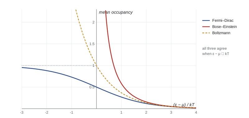
The only difference is the sign in the denominator, and yet the two behave completely differently at low energy. The Fermi–Dirac occupancy can never exceed 1: well below \(\mu\) every orbital is full, well above it every orbital is nearly empty, and the step between them has a width of a few \(kT\). The Bose–Einstein occupancy diverges as \(\varepsilon\) approaches \(\mu\) from above, so for bosons \(\mu\) must lie below the lowest orbital energy, and orbitals just above \(\mu\) can hold enormous numbers of particles. Both distributions approach the Boltzmann form \(e^{-(\varepsilon - \mu)/kT}\) when \(\varepsilon - \mu \gg kT\), because then the occupancy is so small that the exclusion principle (or the bosons' tendency to bunch) never comes into play.

When is a gas quantum?

The Boltzmann limit applies when every orbital's occupancy is much less than 1, which requires \(e^{\mu/kT} \ll 1\). Lesson 7 showed that for a classical ideal gas \(e^{\mu/kT} = n\lambda^3\) (with \(Z_{\text{int}} = 1\)), so the criterion is

In words: the gas is classical when the average volume per particle is much larger than the cube of the thermal wavelength, so that the particles' wave packets rarely overlap. The first part of the program evaluates \(n\lambda^3\) for several systems. Nitrogen at room conditions has \(n\lambda^3 \approx 2 \times 10^{-7}\): thoroughly classical. Helium gas at its boiling point reaches 0.13, where quantum corrections of a few parts in a hundred are noticeable. Liquid helium near 2 K has \(n\lambda^3 \approx 4\), deep in the quantum regime, and indeed it becomes a superfluid. Electrons in copper at room temperature have \(n\lambda^3\) near 7,000, because their small mass makes \(\lambda\) a few nanometers: the conduction electrons of a metal are an intensely quantum gas, which is the subject of lesson 9.

import math
k = 1.380649e-23; h = 6.62607015e-34; u = 1.66053907e-27; me = 9.1093837e-31

def lam(m, T): return h / math.sqrt(2 * math.pi * m * k * T)

# 1. How quantum is a gas? Compare n with the quantum concentration n_Q = 1/lambda^3
cases = [('N2, 300 K, 1 bar', 28.014 * u, 300.0, 1e5 / (k * 300.0)),
         ('He gas, 4.2 K, 1 bar', 4.0026 * u, 4.2, 1e5 / (k * 4.2)),
         ('liquid He-4, 2.2 K', 4.0026 * u, 2.2, 145.0 / (4.0026 * u)),
         ('electrons in copper, 300 K', me, 300.0, 8.47e28)]
print("Degeneracy parameter n lambda^3 (much less than 1: classical)")
for name, m, T, n in cases:
    print(f"  {name:28}: lambda = {lam(m, T):.3e} m, n lambda^3 = {n * lam(m, T) ** 3:.3e}")

# 2. Occupancy of a single orbital, x = (eps - mu)/kT
print("\nMean occupancy against x = (eps - mu)/kT")
print("    x      FD       BE       MB")
for x in (-2.0, -0.5, 0.01, 0.5, 1.0, 2.0, 4.0):
    fd = 1 / (math.exp(x) + 1)
    be = 1 / (math.exp(x) - 1) if x > 0 else float('nan')
    mb = math.exp(-x)
    print(f"  {x:5}  {fd:7.4f}  {be:7.4f}  {mb:7.4f}")

# 3. Polylogarithm f_{s}(z) = sum z^l / l^s; n lambda^3 = g f_{3/2}(z) for an ideal quantum gas
def f(s, z, sign=1):      # sign = +1 for bosons, -1 for fermions: sum (+/-)^(l+1) z^l / l^s
    tot, l = 0.0, 1
    while True:
        term = (sign ** (l + 1)) * z ** l / l ** s
        tot += term
        if abs(term) < 1e-14 or l > 200000: break
        l += 1
    return tot
z1 = f(1.5, 1.0, 1)
print(f"\nzeta(3/2) = f_3/2(1): series stopped at 200001 terms gives {z1:.4f}; adding the tail 2/sqrt(L) gives {z1 + 2 / math.sqrt(200001.5):.4f}")
print("Pressure of an ideal quantum gas relative to classical, PV/(NkT) = f_5/2(z)/f_3/2(z)")
for z in (0.01, 0.1, 0.3, 0.6):
    pb = f(2.5, z, 1) / f(1.5, z, 1)
    pf = f(2.5, z, -1) / f(1.5, z, -1)
    nl3b, nl3f = f(1.5, z, 1), f(1.5, z, -1)
    print(f"  z = {z:4}: bosons n lam^3 = {nl3b:.4f}, PV/NkT = {pb:.4f} (series 1 - n lam^3/2^2.5 = {1 - nl3b / 2 ** 2.5:.4f});"
          f" fermions n lam^3 = {nl3f:.4f}, PV/NkT = {pf:.4f}")

Degeneracy parameter n lambda^3 (much less than 1: classical)
  N2, 300 K, 1 bar            : lambda = 1.904e-11 m, n lambda^3 = 1.667e-07
  He gas, 4.2 K, 1 bar        : lambda = 4.258e-10 m, n lambda^3 = 1.331e-01
  liquid He-4, 2.2 K          : lambda = 5.883e-10 m, n lambda^3 = 4.443e+00
  electrons in copper, 300 K  : lambda = 4.303e-09 m, n lambda^3 = 6.751e+03

Mean occupancy against x = (eps - mu)/kT
    x      FD       BE       MB
   -2.0   0.8808      nan   7.3891
   -0.5   0.6225      nan   1.6487
   0.01   0.4975  99.5008   0.9900
    0.5   0.3775   1.5415   0.6065
    1.0   0.2689   0.5820   0.3679
    2.0   0.1192   0.1565   0.1353
    4.0   0.0180   0.0187   0.0183

zeta(3/2) = f_3/2(1): series stopped at 200001 terms gives 2.6079; adding the tail 2/sqrt(L) gives 2.6124
Pressure of an ideal quantum gas relative to classical, PV/(NkT) = f_5/2(z)/f_3/2(z)
  z = 0.01: bosons n lam^3 = 0.0100, PV/NkT = 0.9982 (series 1 - n lam^3/2^2.5 = 0.9982); fermions n lam^3 = 0.0100, PV/NkT = 1.0018
  z =  0.1: bosons n lam^3 = 0.1037, PV/NkT = 0.9816 (series 1 - n lam^3/2^2.5 = 0.9817); fermions n lam^3 = 0.0966, PV/NkT = 1.0171
  z =  0.3: bosons n lam^3 = 0.3383, PV/NkT = 0.9398 (series 1 - n lam^3/2^2.5 = 0.9402); fermions n lam^3 = 0.2725, PV/NkT = 1.0479
  z =  0.6: bosons n lam^3 = 0.7982, PV/NkT = 0.8567 (series 1 - n lam^3/2^2.5 = 0.8589); fermions n lam^3 = 0.5029, PV/NkT = 1.0881

Density of states

To find the properties of a quantum gas, we sum the occupancy over all orbitals. For particles in a large box of volume \(V\), the orbitals are plane waves, and the number of orbitals with momentum magnitude between \(p\) and \(p + dp\) is the phase-space volume \(V \cdot 4\pi p^2dp\) divided by \(h^3\), times a degeneracy \(g_s\) for spin (2 for electrons). With \(\varepsilon = p^2/2m\) this becomes a density of states in energy:

The \(\sqrt\varepsilon\) form is characteristic of non-relativistic particles in three dimensions. For photons and phonons, with \(\varepsilon = cp\), the density of states grows as \(\varepsilon^2\) instead. Sums over orbitals then become integrals:

The first equation, at given \(N\) and \(T\), determines \(\mu\). In general it must be solved numerically, but the integrals have a standard form. Writing \(z = e^{\mu/kT}\), called the fugacity, the results for an ideal quantum gas are

with the upper sign (all terms positive) for bosons and alternating signs for fermions. The functions \(f_s\) are polylogarithms. For small \(z\) only the first term matters, \(f_s(z) \approx z\), and both lines reduce to the classical results \(n\lambda^3 = g_sz\) and \(P = nkT\). The second part of the program sums the series. At \(z = 1\) the boson series for \(f_{3/2}\) converges slowly to \(\zeta(3/2) = 2.612\), the number that will set the Bose–Einstein condensation temperature in lesson 10.

The first quantum correction

Keeping the second term of each series and eliminating \(z\) gives the equation of state to first order in \(n\lambda^3\):

with the minus sign for bosons and the plus sign for fermions. Fermions exert slightly more pressure than a classical gas, as if they repelled each other, and bosons slightly less, as if they attracted. No force is involved: the effect comes purely from the symmetry of the wave function, which makes fermions avoid each other and bosons bunch together. The program confirms the expansion against the full series. For helium-4 gas at its boiling point, \(n\lambda^3 = 0.13\) gives a correction of about 2 parts in 100, comparable to the effect of the real attractive forces between the atoms, which are much larger at that temperature, so the statistical correction is hard to isolate in helium. In electrons and in ultracold atoms, statistics dominates.

Bunching and antibunching

The tendency of bosons to bunch and fermions to avoid each other can be seen directly. In 1956 Robert Hanbury Brown and Richard Twiss found that photons from a star arrive at two detectors with correlated timing, a bunching effect they used to measure stellar diameters. Similar experiments in the 2000s compared ultracold clouds of helium-4 (bosons) and helium-3 (fermions) released from a trap: the bosonic atoms showed an excess of pairs arriving close together, the fermionic atoms a deficit. The occupancy formulas above are the statistical summary of those correlations.