Applications of the canonical ensemble: paramagnets, two-level systems and equipartition

With the partition function in hand, many problems that would be laborious by counting become short exercises. This lesson works through three of the most important. Paramagnets show how a magnetic field competes with thermal agitation, and they lead to Curie's law and to a refrigeration method that reaches the millikelvin range. Two-level systems show a characteristic bump in the heat capacity, the Schottky anomaly, which appears in real materials whenever a small energy gap is present. And the equipartition theorem, which PHYS-261 used as a rule, is proved here from the canonical ensemble, together with a generalization and a clear statement of when it fails.

The spin-half paramagnet

A dipole with magnetic moment \(\mu\) in a field \(B\) has energy \(-\mu B\) when aligned and \(+\mu B\) when anti-aligned. For one dipole, \(Z_1 = e^{\beta\mu B} + e^{-\beta\mu B} = 2\cosh(\beta\mu B)\). The mean moment along the field is

and for \(N\) independent dipoles the magnetization is \(M = N\mu\tanh(\mu B/kT)\). In strong fields or at low temperature, \(\tanh \to 1\) and the sample saturates with every dipole aligned. In weak fields \(\tanh x \approx x\), so \(M \approx N\mu^2B/kT\): the magnetization is proportional to \(B/T\). This is Curie's law, found experimentally by Pierre Curie in 1895. The energy is \(U = -MB\), and the heat capacity, as for any two-level system, shows the Schottky peak discussed below.

For an electron spin, \(\mu\) is the Bohr magneton \(\mu_B = e\hbar/2m_e = 9.274 \times 10^{-24}\) J/T. In a 1 T field at 300 K, \(\mu_BB/kT = 0.0022\): thermal agitation wins easily and the magnetization is only about two parts in a thousand of its saturation value. At 1 K the same field gives \(\mu_BB/kT = 0.67\) and a substantial fraction of the spins align. Nuclear moments are about 2,000 times smaller, which is why nuclear magnetic resonance signals are weak and why magnetic resonance imaging uses fields of several tesla.

Larger angular momenta: the Brillouin function

Many paramagnetic ions carry an angular momentum quantum number \(J\) larger than one half. Quantum mechanics (PHYS-372 and PHYS-373) allows the component along the field to take \(2J + 1\) values, \(m_J = -J, \ldots, J\), with energies \(-g\mu_Bm_JB\), where \(g\) is the Landé factor, equal to 2 for a pure spin. The single-ion partition function is a finite geometric series:

Differentiating \(\ln Z_1\) with respect to \(B\) gives the mean moment \(g\mu_BJ\,B_J(x)\), where the Brillouin function is

For \(J = \frac12\) this reduces to \(\tanh x\). For small \(x\) it gives Curie's law in the form \(M = Ng^2\mu_B^2J(J + 1)B/3kT\); the combination \(g\sqrt{J(J + 1)}\) is called the effective moment, and measuring it identifies the magnetic state of an ion. The classical limit \(J \to \infty\) gives the Langevin function \(\coth x - 1/x\) of 1905.

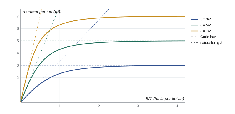
The Brillouin function was tested decisively by Warren Henry in 1952, using salts of chromium (\(J = \frac32\)), iron (\(J = \frac52\)) and gadolinium (\(J = \frac72\)) at liquid-helium temperatures and fields of a few tesla. Plotted against \(B/T\), his measurements at several temperatures fell on single curves that matched the theory closely, confirming both the quantization of angular momentum and the statistical treatment. The first part of the program below computes these curves.

import math

def brillouin(J, x):
    """B_J(x) with x = g muB J B / kT; magnetization / saturation value."""
    if x == 0: return 0.0
    a = (2 * J + 1) / (2 * J)
    c = 1 / (2 * J)
    coth = lambda y: 1 / math.tanh(y)
    return a * coth(a * x) - c * coth(c * x)

muB, k = 9.274e-24, 1.380649e-23
print("Moment per ion (in Bohr magnetons) for spin-only ions, g = 2, against B/T")
print("  B/T (T/K)   J=3/2 (Cr3+)  J=5/2 (Fe3+)  J=7/2 (Gd3+)")
for BT in (0.5, 1.0, 2.0, 4.0):
    y = muB * BT / k                     # muB B / kT
    row = [2 * J * brillouin(J, 2 * J * y) for J in (1.5, 2.5, 3.5)]
    print(f"  {BT:8}     " + "        ".join(f"{r:6.3f}" for r in row))
print("  saturation values g J: 3, 5, 7")
print(f"  check: B_1/2(x) = tanh(x)? B_1/2(1) = {brillouin(0.5, 1.0):.4f}, tanh(1) = {math.tanh(1):.4f}")
y = muB * 0.01 / k
print(f"  weak field (B/T = 0.01 T/K), J = 7/2: moment {7 * brillouin(3.5, 7 * y):.5f}, "
      f"Curie law g^2 J(J+1) y/3 = {4 * 3.5 * 4.5 * y / 3:.5f}")

# Schottky anomaly: two-level system with gap eps; find the heat-capacity peak
def C(t):           # C/(N k) with t = kT/eps
    x = 1 / t
    return x * x * math.exp(x) / (1 + math.exp(x)) ** 2
best = max((i / 100000 for i in range(1000, 200000)), key=C)
print(f"\nSchottky peak: kT/eps = {best:.4f}, C/(Nk) = {C(best):.4f}")

# Adiabatic demagnetization of an ideal spin-1/2 paramagnet: S depends only on B/T
Ti, Bi, Bf = 1.0, 2.0, 0.01        # K, T (tesla), residual internal field in tesla
Tf = Ti * Bf / Bi
x = muB * Bi / (k * Ti)
s = math.log(2 * math.cosh(x)) - x * math.tanh(x)     # S/(N k)
print(f"\nDemagnetization: start {Ti} K in {Bi} T (x = {x:.3f}, S/Nk = {s:.4f} of max {math.log(2):.4f})")
print(f"  reduce field to {Bf} T at constant S: final temperature {Tf * 1000:.1f} mK")

# Generalized equipartition: <V> = kT/n for V = a|x|^n, checked by quadrature (kT = 1)
print("\nEquipartition for V = |x|^n at kT = 1")
for n in (2, 4, 6):
    xs = [i * 1e-3 for i in range(-8000, 8001)]
    w = [math.exp(-abs(x) ** n) for x in xs]
    V = sum(abs(x) ** n * wi for x, wi in zip(xs, w)) / sum(w)
    print(f"  n = {n}: <V> = {V:.4f}, prediction 1/n = {1 / n:.4f}")

Moment per ion (in Bohr magnetons) for spin-only ions, g = 2, against B/T
  B/T (T/K)   J=3/2 (Cr3+)  J=5/2 (Fe3+)  J=7/2 (Gd3+)
       0.5      1.496         3.129         4.986
       1.0      2.331         4.298         6.294
       2.0      2.854         4.854         6.854
       4.0      2.991         4.991         6.991
  saturation values g J: 3, 5, 7
  check: B_1/2(x) = tanh(x)? B_1/2(1) = 0.7616, tanh(1) = 0.7616
  weak field (B/T = 0.01 T/K), J = 7/2: moment 0.14103, Curie law g^2 J(J+1) y/3 = 0.14106

Schottky peak: kT/eps = 0.4168, C/(Nk) = 0.4392

Demagnetization: start 1.0 K in 2.0 T (x = 1.343, S/Nk = 0.2372 of max 0.6931)
  reduce field to 0.01 T at constant S: final temperature 5.0 mK

Equipartition for V = |x|^n at kT = 1
  n = 2: <V> = 0.5000, prediction 1/n = 0.5000
  n = 4: <V> = 0.2500, prediction 1/n = 0.2500
  n = 6: <V> = 0.1667, prediction 1/n = 0.1667

Cooling by demagnetization

For an ideal paramagnet, the partition function depends on \(B\) and \(T\) only through \(B/T\), so the entropy does too. If the sample is magnetized at low temperature while in contact with a bath, its entropy falls as the spins align, and the bath carries away the heat. If the sample is then isolated and the field reduced slowly, the entropy stays constant, so \(B/T\) stays constant: reducing the field by a factor of 200 reduces the temperature by a factor of 200. Proposed by Peter Debye and William Giauque independently in 1926 and demonstrated by Giauque and MacDougall in 1933, adiabatic demagnetization was the first route below 1 K. In practice the cooling stops when the field reaches the small internal field produced by interactions between the spins, as the program's example of 2 T falling to an effective 0.01 T illustrates: 1 K becomes 5 mK. Demagnetizing nuclear spins, whose interactions are weaker still, has reached microkelvin temperatures.

Two-level systems and the Schottky anomaly

Any system with two low-lying states separated by an energy \(\varepsilon\), far below all other excitations, behaves like the spin-half paramagnet. Examples include magnetic ions whose levels are split by the crystal field, tunneling defects in glasses and molecules that can sit in one of two configurations. With energies 0 and \(\varepsilon\),

The heat capacity vanishes at low temperature, because the excited state is out of reach, and also at high temperature, because both states are then equally occupied and adding energy cannot change the populations much more. In between it has a peak, at \(kT = 0.417\varepsilon\), of height \(0.439Nk\), as the program finds. This Schottky anomaly, named for Walter Schottky who analyzed it in 1922, is a signature used to measure small energy gaps: the position of the peak gives \(\varepsilon\), and its height counts the number of two-level systems.

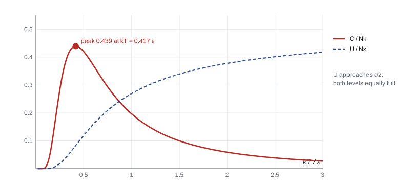
Unlike a gas or a solid, whose heat capacities level off at high temperature, a two-level system cannot absorb unlimited energy: its energy is bounded by \(N\varepsilon\). That is the same bound that allows negative temperatures in lesson 3.

The equipartition theorem

In classical statistical mechanics, the partition function of a particle is an integral over phase space. Suppose the energy contains a term that is quadratic in one coordinate or momentum, \(E = cq^2\), independent of the other variables. Then the average of that term is

Each quadratic degree of freedom carries an average energy of \(\frac12 kT\), whatever the coefficient \(c\). This is the equipartition theorem. A monatomic gas has three quadratic momentum terms, so \(U = \frac32 NkT\); a diatomic gas adds two rotational terms, giving \(\frac52 NkT\); a solid has three kinetic and three potential terms per atom, giving \(3NkT\) and the Dulong–Petit heat capacity.

The same calculation for a term \(c|q|^n\) gives \(\overline{c|q|^n} = kT/n\), a generalized equipartition theorem that the last part of the program confirms by numerical integration. A particle in a quartic well, for example, has a mean potential energy of \(kT/4\), not \(kT/2\). An even more general form, \(\overline{q\,\partial E/\partial q} = kT\), holds for any coordinate whose Boltzmann factor vanishes at the ends of its range, and it underlies the virial theorem.

When equipartition fails

Equipartition is a classical result, and it fails whenever the quantum spacing of a degree of freedom's levels is large compared with \(kT\). A degree of freedom with level spacing \(\varepsilon\) contributes its full share only when \(kT \gg \varepsilon\); when \(kT \ll \varepsilon\), it is frozen in its ground state and contributes nothing. This was one of the great puzzles of nineteenth-century physics. Maxwell worried in 1875 that diatomic molecules must have vibrational and many other internal degrees of freedom, yet the measured heat capacity of air showed only five quadratic terms. The resolution came only with quantum mechanics: at room temperature the vibrational quanta of nitrogen and oxygen are about ten times \(kT\), so vibration is frozen out, while rotational quanta are much smaller than \(kT\), so rotation contributes fully. Lesson 6 calculates these contributions in detail. The failure of equipartition for the electromagnetic field, which gave the ultraviolet catastrophe, is treated in lesson 10.