Microstates, multiplicity and the fundamental postulate

Everything in statistical mechanics begins with counting. To predict what a system will do, we count the microstates that belong to each of its possible macrostates; the macrostate with the most microstates is the one we will observe. This lesson develops the counting for three model systems that run through the whole course, the two-state paramagnet, the Einstein solid and the ideal gas, and then uses the counting to show how two systems in contact share their energy. PHYS-261 introduced the Einstein solid and computed one example of shared energy numerically. Here we work out the general pattern, see why the result becomes sharp as systems grow, and examine the assumption that makes it all work.

The two-state paramagnet

The simplest system with interesting statistics is a collection of \(N\) independent magnetic dipoles, each of which can point only up or down along an applied magnetic field. Physically, these might be the spins of unpaired electrons in a salt, or the nuclear spins in a sample for magnetic resonance. A microstate is a list saying which dipoles point up. The macrostate is specified by the number \(N_\uparrow\) that point up, which fixes the total magnetic moment and the energy in the field. The multiplicity of the macrostate is the number of ways of choosing which \(N_\uparrow\) of the \(N\) dipoles are up:

The total number of microstates is \(2^N\), and the multiplicity is largest at \(N_\uparrow = N/2\). Using Stirling's approximation with \(N_\uparrow = N(1 + x)/2\), where \(x\) is the fractional magnetization, gives

which equals \(N\ln 2\) at \(x = 0\) and falls to zero at \(x = \pm 1\). Expanding near the peak, \(\ln\Omega \approx N\ln 2 - Nx^2/2\), so the multiplicity is a Gaussian in \(x\) with width \(1/\sqrt N\), the same \(1/\sqrt N\) seen in lesson 1.

The Einstein solid

Einstein's 1907 model of a solid treats each atom as three independent quantum harmonic oscillators, each with the same frequency \(\omega\), so that each oscillator has energy levels \(n\hbar\omega\) above its ground state (the zero-point energy is a constant we can ignore). A solid of \(N\) oscillators with total energy \(U = q\varepsilon\), where \(\varepsilon = \hbar\omega\), has \(q\) quanta of energy to share among \(N\) oscillators. The number of ways to do this is a classic counting problem: line up the \(q\) quanta as dots and separate them into \(N\) groups with \(N - 1\) bars. Every arrangement of \(q\) dots and \(N - 1\) bars is a distinct microstate, so

For large \(N\) and \(q\), Stirling's approximation gives \(\ln\Omega \approx (q + N)\ln(q + N) - q\ln q - N\ln N\). In the high-energy limit \(q \gg N\) this simplifies to \(\Omega \approx (eq/N)^N\), and in the low-energy limit \(q \ll N\) to \(\Omega \approx (eN/q)^q\). Either way the multiplicity grows as a large power of the energy, a pattern that turns out to be universal.

The ideal gas

For a monatomic ideal gas of \(N\) atoms in a box of volume \(V\), the microstates are not discrete in classical mechanics, so counting requires a rule. Quantum mechanics supplies it. Each atom is a particle in a box, with states labeled by three quantum numbers, and the number of states with momentum in a small range is the volume of position-momentum space (phase space) divided by \(h^3\), as follows from the box states of PHYS-372. Lesson 3 carries out this count. The result has the form

with \(f(N)\) a function of \(N\) alone. Each atom contributes a factor of \(V\), because it can be anywhere in the box, and the energy appears to the power \(3N/2\), half the number of momentum components. The exponents are of order \(N\), which is why the multiplicity is such a steep function of energy and volume.

Two systems in contact

Now let two Einstein solids, A with \(N_A\) oscillators and B with \(N_B\), share a total of \(q\) quanta. Energy can flow between them, slowly compared with the time it takes each solid to rearrange its own quanta, so we can treat each solid as being in equilibrium internally. A macrostate of the combined system is specified by \(q_A\), the number of quanta in A, and its multiplicity is the product

because every microstate of A can be combined with every microstate of B. According to the fundamental postulate, all microstates of the combined isolated system are equally likely, so the probability of the macrostate \(q_A\) is proportional to \(\Omega_{\text{total}}(q_A)\). For small solids the distribution is broad. As the solids grow, it narrows dramatically around its peak.

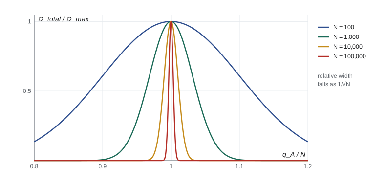
The program below computes the distribution exactly, using logarithms of factorials so that no overflow occurs. It finds the most probable division, the mean, the width and the probability that solid A holds at least one part in a hundred more than its fair share of the energy.

import math

def ln_omega(N, q):
    """ln of the multiplicity of an Einstein solid: N oscillators, q quanta."""
    return math.lgamma(q + N) - math.lgamma(q + 1) - math.lgamma(N)

def share(NA, NB, q):
    """Distribution of q_A when two solids share q quanta: peak, width, tail."""
    lw = [ln_omega(NA, a) + ln_omega(NB, q - a) for a in range(q + 1)]
    top = max(lw)
    w = [math.exp(x - top) for x in lw]
    tot = sum(w)
    mean = sum(a * wi for a, wi in enumerate(w)) / tot
    var = sum((a - mean) ** 2 * wi for a, wi in enumerate(w)) / tot
    return mean, math.sqrt(var), lw, top

print("Two identical Einstein solids sharing q = 2N quanta")
for N in (100, 1000, 10000, 100000):
    mean, sd, lw, top = share(N, N, 2 * N)
    # probability that solid A holds 1 part in 100 more than its fair share or more
    cut = int(1.01 * N)
    tail = sum(math.exp(x - top) for x in lw[cut:]) / sum(math.exp(x - top) for x in lw)
    print(f"  N = {N:>6}: most likely q_A = {lw.index(top)}, mean {mean:.1f}, "
          f"width {sd:.2f}, relative width {sd / mean:.2e}, P(q_A >= 1.01 N) = {tail:.2e}")

print("\nUnequal solids: N_A = 3000, N_B = 1000 sharing q = 4000 quanta")
mean, sd, lw, top = share(3000, 1000, 4000)
print(f"  most likely q_A = {lw.index(top)} (quanta per oscillator in A: {lw.index(top) / 3000:.3f}, "
      f"in B: {(4000 - lw.index(top)) / 1000:.3f})")

# Gaussian estimate of the width for large N: relative width ~ 1/sqrt(N) scaling
print("\nScaling check: width times sqrt(N)/N should settle down")
for N in (1000, 10000, 100000):
    mean, sd, lw, top = share(N, N, 2 * N)
    print(f"  N = {N:>6}: (width / N) x sqrt(N) = {sd / N * math.sqrt(N):.4f}")

Two identical Einstein solids sharing q = 2N quanta
  N =    100: most likely q_A = 100, mean 100.0, width 9.98, relative width 9.98e-02, P(q_A >= 1.01 N) = 4.80e-01
  N =   1000: most likely q_A = 1000, mean 1000.0, width 31.61, relative width 3.16e-02, P(q_A >= 1.01 N) = 3.82e-01
  N =  10000: most likely q_A = 10000, mean 10000.0, width 100.00, relative width 1.00e-02, P(q_A >= 1.01 N) = 1.60e-01
  N = 100000: most likely q_A = 100000, mean 100000.0, width 316.23, relative width 3.16e-03, P(q_A >= 1.01 N) = 7.87e-04

Unequal solids: N_A = 3000, N_B = 1000 sharing q = 4000 quanta
  most likely q_A = 3001 (quanta per oscillator in A: 1.000, in B: 0.999)

Scaling check: width times sqrt(N)/N should settle down
  N =   1000: (width / N) x sqrt(N) = 0.9998
  N =  10000: (width / N) x sqrt(N) = 1.0000
  N = 100000: (width / N) x sqrt(N) = 1.0000

The width of the distribution is \(\sqrt N\) quanta for these solids, so the relative width is \(1/\sqrt N\): 0.1 for 100 oscillators, 0.003 for 100,000. The probability that solid A holds 1 part in 100 more than half of the energy falls from about one half to under one in a thousand over this range. For a macroscopic solid with \(N \approx 10^{23}\), the relative width would be about \(3 \times 10^{-12}\), and the probability of a deviation of one part in a hundred would be roughly \(e^{-10^{19}}\). The energy divides itself in the most probable way, and stays there. For unequal solids, the third part of the output shows the division puts equal energy per oscillator in each, which is the condition for equal temperature, as lesson 3 will show.

Why the peak is sharp

The sharpness has a simple origin. Write \(\Omega_{\text{total}} = \exp[\ln\Omega_A + \ln\Omega_B]\). Each logarithm is of order \(N\) and is a smooth function of \(q_A\). At the peak the sum has zero slope, and its curvature is of order \(1/N\) per quantum squared, so expanding to second order about the peak \(\bar q_A\) gives

The peak sits at a value of order \(N\), with a width of order \(\sqrt N\). This structure, an exponent of order \(N\) whose second derivative is of order \(1/N\), appears in every macroscopic system, and it is the mathematical reason thermodynamics works. Lesson 4 will connect the width to the heat capacity, through the formula \(\sigma_E^2 = kT^2C\).

The fundamental postulate, examined

The calculation above assumed that all microstates of the combined system are equally likely. Is that justified? There are three ways to think about it.

There are systems for which the postulate fails on practical time scales. A glass is a liquid that has fallen out of equilibrium: its atoms are frozen into one disordered arrangement and cannot reach the others in any reasonable time. Hydrogen gas, as lesson 6 will show, has two forms whose interconversion is so slow that they behave like separate species. In such cases we apply the postulate to the microstates that are actually accessible, and the resulting statistics still work.

Distinguishable and indistinguishable particles

In the Einstein solid the oscillators are fixed to lattice sites, so they are distinguishable by position: quanta in oscillator 3 and quanta in oscillator 7 make different microstates. The quanta themselves are not labeled, which is why we count arrangements of identical dots. In a gas the atoms move freely and are identical, so exchanging two atoms does not produce a new microstate. Counting them as labeled overcounts by a factor of \(N!\), the number of ways to permute the labels. Ignoring this factor gives an entropy that is not extensive, a famous puzzle that lesson 3 resolves. Quantum mechanics makes the point sharper: identical particles are truly indistinguishable, and this leads to the Bose and Fermi statistics of lessons 8 to 10.