The statistical interpretation: microstates, multiplicity and Boltzmann's entropy

Thermodynamics defines entropy through heat and temperature and proves that it never decreases in an isolated system, but it does not say what entropy is. Boltzmann's answer, that entropy measures the number of microscopic arrangements consistent with what we observe, is one of the great ideas of physics. This lesson develops it in the simplest model where everything can be counted exactly, the Einstein solid. We count microstates, watch two solids share energy, see why the most probable division of energy becomes a certainty for large systems, and recover temperature, the second law and the heat capacity from the counting alone. We then state the corresponding result for the ideal gas, the Sackur–Tetrode equation.

The fundamental assumption

Consider an isolated system with fixed energy \(U\), volume \(V\) and number of particles \(N\). Quantum mechanics says that such a system has a finite, though enormous, number of accessible microstates. The fundamental assumption of statistical mechanics is that in equilibrium all accessible microstates are equally probable. It cannot be derived from mechanics in general, though it can be made plausible: if the dynamics carries the system through all accessible states over time and has no reason to favor any, the long-time average should treat them equally. Its justification is that its consequences agree with experiment in every case that has been tested.

The number of microstates corresponding to a macrostate is its multiplicity, \(\Omega\). By the fundamental assumption, the probability of a macrostate is proportional to its multiplicity. Equilibrium is the macrostate of maximum multiplicity, and fluctuations away from it are suppressed in proportion to how fast the multiplicity falls.

Counting the states of an Einstein solid

In Einstein's model of lesson 5, a solid of \(N/3\) atoms is a collection of \(N\) independent quantum oscillators, all with the same frequency. Each oscillator has energy levels \(\varepsilon(j + \frac12)\) with \(j = 0, 1, 2, \ldots\), so above the ground state the solid's energy is \(q\varepsilon\), where \(q\) is the total number of energy quanta shared among the oscillators. A microstate is a list of how many quanta each oscillator has. How many lists add up to \(q\)?

Represent each quantum by a dot and separate the oscillators by \(N - 1\) bars. For example, with \(N = 4\) and \(q = 5\), the arrangement \(\bullet\bullet|\bullet||\bullet\bullet\) gives two quanta to the first oscillator, one to the second, none to the third and two to the fourth. Every microstate corresponds to exactly one arrangement of \(q\) dots and \(N - 1\) bars in a row, and every such arrangement is a microstate. Choosing which \(q\) of the \(q + N - 1\) positions hold dots gives

For \(N = 4\) and \(q = 5\), that is \(\binom{8}{5} = 56\) microstates. The numbers grow explosively: a solid of 300 oscillators with 100 quanta has about \(1.7 \times 10^{96}\) microstates.

Two solids in thermal contact

Now let two Einstein solids, A with \(N_A\) oscillators and B with \(N_B\), share \(q\) quanta, so that \(q_A + q_B = q\). Energy can pass between them, slowly enough that each solid is internally in equilibrium; this is a model of thermal contact. The combined system is isolated, so by the fundamental assumption all of its microstates are equally likely. The number of microstates with \(q_A\) quanta in A is \(\Omega_A(q_A)\,\Omega_B(q - q_A)\), and the probability of that division of energy is this product divided by the total, \(\Omega(N_A + N_B, q)\).

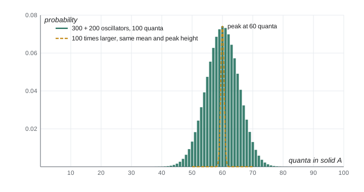
import math, random

def omega(N, q):                        # multiplicity of an Einstein solid
    return math.comb(q + N - 1, q)

# Two Einstein solids sharing q_total quanta
NA, NB, q_total = 300, 200, 100
total = omega(NA + NB, q_total)
best = max(range(q_total + 1), key=lambda qA: omega(NA, qA) * omega(NB, q_total - qA))
print(f"solids A ({NA} oscillators) and B ({NB}), {q_total} quanta shared")
print(f"total microstates {float(total):.4e}")
print(" qA    Omega_A*Omega_B    probability")
for qA in (0, 20, 40, 50, 60, 70, 80, 100):
    w = omega(NA, qA) * omega(NB, q_total - qA)
    print(f"{qA:3d}    {float(w):14.4e}    {w / total:.3e}")
print(f"most probable qA = {best}  (energy shared in proportion to size: {q_total * NA / (NA + NB):.0f})")

# Entropy S/k = ln Omega and temperature 1/T = dS/dU, in units of the quantum energy
def S(N, q): return math.log(omega(N, q))
qA = best
inv_TA = S(NA, qA + 1) - S(NA, qA - 1)
inv_TB = S(NB, q_total - qA + 1) - S(NB, q_total - qA - 1)
print(f"at equilibrium: kT_A/eps = {2 / inv_TA:.3f}, kT_B/eps = {2 / inv_TB:.3f}")

# Width of the peak shrinks as the solids grow
for scale in (1, 10, 100):
    na, nb, qt = NA * scale, NB * scale, q_total * scale
    logw = [math.lgamma(q + na) - math.lgamma(q + 1) - math.lgamma(na) +
            math.lgamma(qt - q + nb) - math.lgamma(qt - q + 1) - math.lgamma(nb) for q in range(qt + 1)]
    mx = max(logw); w = [math.exp(x - mx) for x in logw]; Z = sum(w)
    mean = sum(q * p for q, p in enumerate(w)) / Z
    sd = math.sqrt(sum((q - mean)**2 * p for q, p in enumerate(w)) / Z)
    print(f"scale x{scale:3d}: relative width of the qA distribution {sd / mean:.4f}")

# Stirling's approximation for ln N!
for n in (10, 100, 1000, 10**6):
    exact = math.lgamma(n + 1)
    print(f"ln {n}! = {exact:.4f}; N ln N - N = {n * math.log(n) - n:.4f}; "
          f"with 0.5 ln(2 pi N): {n * math.log(n) - n + 0.5 * math.log(2 * math.pi * n):.4f}")

# Random exchange of single quanta drives an initially lopsided split to the peak
rnd = random.Random(261)
osc = [1] * 100 + [0] * 400            # all 100 quanta start in the first 100 oscillators (in A)
for step in range(200001):
    if step % 40000 == 0:
        print(f"step {step:6d}: quanta in A = {sum(osc[:NA])}")
    i, j = rnd.randrange(500), rnd.randrange(500)
    if osc[i] > 0:
        osc[i] -= 1; osc[j] += 1

solids A (300 oscillators) and B (200), 100 quanta shared
total microstates 9.2618e+115
 qA    Omega_A*Omega_B    probability
  0        2.7722e+81    2.993e-35
 20       5.6549e+102    6.106e-14
 40       8.0919e+111    8.737e-05
 50       1.2271e+114    1.325e-02
 60       6.8663e+114    7.414e-02
 70       1.2084e+114    1.305e-02
 80       3.6814e+111    3.975e-05
100        1.6814e+96    1.815e-20
most probable qA = 60  (energy shared in proportion to size: 60)
at equilibrium: kT_A/eps = 0.561, kT_B/eps = 0.563
scale x  1: relative width of the qA distribution 0.0894
scale x 10: relative width of the qA distribution 0.0283
scale x100: relative width of the qA distribution 0.0089
ln 10! = 15.1044; N ln N - N = 13.0259; with 0.5 ln(2 pi N): 15.0961
ln 100! = 363.7394; N ln N - N = 360.5170; with 0.5 ln(2 pi N): 363.7385
ln 1000! = 5912.1282; N ln N - N = 5907.7553; with 0.5 ln(2 pi N): 5912.1281
ln 1000000! = 12815518.3847; N ln N - N = 12815510.5580; with 0.5 ln(2 pi N): 12815518.3847
step      0: quanta in A = 100
step  40000: quanta in A = 61
step  80000: quanta in A = 56
step 120000: quanta in A = 57
step 160000: quanta in A = 62
step 200000: quanta in A = 64

The most probable division gives 60 quanta to A and 40 to B, in proportion to the number of oscillators, so on average each oscillator in both solids has the same energy. The probability that A holds all 100 quanta, which might be our starting condition if A were initially hot and B at absolute zero, is about \(10^{-20}\); the probability that A holds none is \(10^{-35}\). Even for these tiny solids, about 95% of the probability lies within ten quanta of the peak, two standard deviations. Making the solids 100 times larger shrinks the relative width of the peak by a factor of 10, as the \(1/\sqrt N\) scaling of lesson 1 predicts; for macroscopic solids with \(10^{23}\) oscillators the relative width is a few parts in \(10^{12}\) and the most probable division is, for all practical purposes, the only one. The random exchange simulation at the end starts with all 100 quanta crowded into A and moves single quanta between randomly chosen oscillators; within 40 000 moves the number in A has fallen to about 60, around which it then fluctuates by a few quanta.

This is the second law at work. Heat flows from the hot solid to the cold one not because any force drives it, but because there are vastly more microstates with the energy shared than with it concentrated, and random exchanges carry the system from the few to the many. Once there, it stays, because the chance of returning is negligible.

Boltzmann's entropy

Multiplicities of independent systems multiply, while entropies should add. The logarithm turns products into sums, which led Boltzmann to define

The entropy of the combined system is then \(S_A + S_B\), and maximizing \(\Omega_A\Omega_B\) is the same as maximizing the total entropy: the second law becomes the statement that an isolated system moves to its macrostate of greatest multiplicity. Max Planck first wrote the equation in this form, with the constant \(k\), in 1900; Boltzmann had expressed the same idea in 1877 in terms of the probability of a state.

At the most probable division, the product \(\Omega_A(q_A)\Omega_B(q - q_A)\) is at its maximum, so its logarithm has zero derivative with respect to \(q_A\):

In equilibrium the two solids have equal values of \(\partial S/\partial U\). That is the defining property of temperature, and comparing with the thermodynamic relation \(dU = T\,dS\) at fixed volume identifies

When energy flows from a body with smaller \(\partial S/\partial U\) to one with larger, the total entropy rises, so heat flows from high \(T\) to low \(T\), as it must. In the program, finite differences of \(\ln\Omega\) at the equilibrium division give \(kT/\varepsilon \approx 0.56\) for both solids.

Stirling's approximation and the large-system limit

For large numbers, factorials are handled with Stirling's approximation, \(\ln N! \approx N\ln N - N\), or more accurately \(N\ln N - N + \frac12\ln(2\pi N)\). The program shows that the simple form is off by 4 in 5912 for \(N = 1000\), and the improved form is essentially exact; for \(N = 10^{23}\) the correction term is utterly negligible. Applying it to the Einstein solid in the high-temperature limit, where \(q \gg N\), gives

Then \(1/T = \partial S/\partial U = (1/\varepsilon)\,\partial S/\partial q = Nk/(q\varepsilon)\), so \(U = q\varepsilon = NkT\). Each oscillator has average energy \(kT\), and the heat capacity is \(Nk\), which is \(3R\) per mole of atoms: the Dulong–Petit law, recovered purely by counting. Keeping the exact multiplicity instead of the approximation reproduces Einstein's full formula, including the fall at low temperature.

The ideal gas and the Sackur–Tetrode equation

For an ideal monatomic gas the microstates are the quantum states of \(N\) particles in a box of volume \(V\) with total energy \(U\). Counting them requires the quantum mechanics of a particle in a box and the geometry of spheres in \(3N\) dimensions, and one more ingredient: identical particles are indistinguishable, so exchanging two of them does not produce a new microstate, and the count must be divided by \(N!\). The result, found by Otto Sackur and Hugo Tetrode independently in 1912, is

Differentiating with respect to \(U\) gives \(U = \frac32 NkT\), and with respect to \(V\), using \(P/T = (\partial S/\partial V)_U\), gives \(PV = NkT\): the ideal gas law emerges from counting. The dependence on \(V\) reproduces the entropy changes of lesson 8, \(Nk\ln(V_2/V_1)\) for an isothermal or free expansion, and the factor \(1/N!\) makes the entropy extensive and resolves the Gibbs paradox: mixing two samples of the same gas gives no entropy change, while mixing different gases gives \(2Nk\ln 2\). Planck's constant appears, showing that even this classical-looking result depends on quantum mechanics for its absolute value. For argon at 298 K and 100 kPa it gives 154.8 J/(mol K), in agreement with the value measured calorimetrically from heat capacities and latent heats starting near absolute zero, a striking check of both statistical mechanics and the third law.