Type curves and unconventional forecasting

The remaining four Phase 2 wells and the six north flank locations have no production at all, so they cannot be forecast by decline analysis. They will be drilled with laterals of about 9,800 feet, close to two miles and longer than most of the existing wells, using the latest completion design. Their forecasts must come from the 14 producing horizontals in the area, combined into type curves. Diane calls type curves “the most powerful and most misused tool in the building”, because a type curve built carelessly from the wrong wells can add or remove millions of dollars of value with no one noticing. This lesson covers how type curves are built, normalized and turned into probabilistic forecasts for undeveloped locations.

What a type curve is

A type curve, often called a type well, is a representative production profile for a group of wells expected to perform alike. It is built from the production histories of analog wells, aligned to a common start, normalized for differences in design, and summarized as an average or as percentiles. In resource plays, where the reservoir is continuous over large areas and well results depend mainly on completion design and position, type curves are the standard way of forecasting undeveloped locations and the basis for development planning, budgets and acquisitions.

A type curve is a statistical statement about a population of wells, not a forecast for one particular well. Individual wells in the same play commonly differ by a factor of two or more in their first-year production, so any single new well may land well above or below the curve. What the curve must do is describe that spread correctly, so that a program of many wells delivers what the curve predicts on average and the reserves categories carry the right levels of confidence.

Selecting the analog wells

The choice of analogs matters more than any later calculation. Analog wells should be in the same geological area, landed in the same zone, and completed with a similar design: stage spacing, proppant per unit length, fluid type and cluster design all affect results. Vintage matters, because completion practice has changed rapidly; wells completed five years ago with half the current proppant intensity are poor analogs for next year's wells, unless their results are adjusted. The evaluator should also consider spacing: a well drilled next to an older, depleted parent well often performs worse than the parent did, so a set of analogs that are all parent wells will overstate the results of infill locations.

Several biases can creep in. Survivorship bias occurs when poorly performing wells are left out, for example because they were sold, shut in or recompleted. Selection bias occurs when the analogs are chosen because they are good. And time bias occurs when only wells with long histories are used, which tends to select older vintages. The SPEE monographs on undeveloped reserves in resource plays recommend documenting the selection criteria, using all wells that meet them, and checking that the sample is large enough for the spread it shows; plays with wide variability need more wells to define the distribution.

Normalization and alignment

Each analog history is first shifted in time so that month one is its first full month of production; calendar dates are discarded. The histories are then normalized for known design differences, most commonly lateral length, so that the curve describes production per meter or per foot of lateral. Normalizing by proppant mass or by the number of stages is also used where these vary widely. Normalization assumes that production scales with the normalizing variable; for lateral length this is roughly true, but longer laterals often deliver somewhat less per unit length because of friction, cleanup and completion efficiency at the toe, so many evaluators apply a scaling exponent below 1 or check the relationship against the data.

A practical problem is that wells have histories of different lengths. Averaging the rates of whichever wells have data in each month gives a curve that is increasingly dominated, at late times, by the oldest and often best wells. The usual remedy is to forecast every well individually to the end of its life with decline curves first, then build the type curve from the forecasts, so that every well contributes over the whole profile.

The distribution of well results

The results of wells in a play are usually well described by a lognormal distribution: most wells cluster around a central value, with a long tail of strong performers. On a probability plot, with the logarithm of the result on one axis and the cumulative probability on a normal scale on the other, lognormal data fall on a straight line. The slope of that line gives the spread, often summarized as the ratio of P10 to P90, and the line provides the percentile values even when the sample is small.

The difference between the median and the mean is important for development planning. For a lognormal distribution the mean exceeds the median by the factor e^(σ²/2), where σ is the standard deviation of the natural logarithm. A company drilling many wells receives, on average, the mean, so the best estimate for a large program should be built on the mean type curve, while the median type curve describes a typical single well. For narrow distributions such as this pool the difference is small; for wide distributions it can be 20 percent or more.

The script below takes the first-twelve-month oil volumes of the 14 producing horizontals, normalizes them by lateral length, computes empirical and lognormal percentiles, and builds P90, P50 and P10 type wells for a 9,800 foot lateral. The ratio of EUR to first-year volume, 4.3, comes from the decline analysis of Lesson 4.

# Type curves: normalize first-year volumes by lateral length and build P90/P50/P10 type wells for Phase 2.
import math
SI = False     # True: m and m3, False: ft and bbl
# 14 producing horizontals: (lateral length, first-12-month oil); metric values, converted for the US case
wells = [(1600, 7900), (1600, 6400), (1800, 9100), (1550, 5200), (2000, 10800), (1600, 7300), (1800, 6600),
         (2400, 12900), (1600, 8400), (1700, 5900), (2400, 10700), (1800, 9900), (2000, 7700), (1600, 7100)]
L_ft, V_bbl = 3.2808, 6.2898
lat = [l if SI else l * L_ft * 1.25 for l, _ in wells]        # the US wells have longer laterals (illustrative)
vol = [v if SI else v * V_bbl * 2.0 for _, v in wells]        # and a more productive Bakken completion
per = sorted(v / l for v, l in zip(vol, lat))       # first-year oil per meter (or foot) of lateral
n = len(per)
def pctl(xs, p):                                    # P90 = 90 percent exceed, using linear interpolation on ranks
    r = (1 - p) * (len(xs) - 1); i = int(r); f = r - i
    return xs[i] * (1 - f) + xs[min(i + 1, len(xs) - 1)] * f
u = "m3 per m" if SI else "bbl per ft"
logs = [math.log(x) for x in per]; mu = sum(logs) / n; sd = (sum((x - mu) ** 2 for x in logs) / (n - 1)) ** 0.5
print(f"{n} wells, normalized first-year oil: min {per[0]:.2f}, max {per[-1]:.2f} {u}")
print(f"empirical P90 {pctl(per, 0.9):.2f}  P50 {pctl(per, 0.5):.2f}  P10 {pctl(per, 0.1):.2f} {u}")
z = 1.2816
p90, p50, p10 = math.exp(mu - z * sd), math.exp(mu), math.exp(mu + z * sd)
print(f"lognormal fit:  P90 {p90:.2f}  P50 {p50:.2f}  P10 {p10:.2f}  (P10/P90 = {p10 / p90:.2f})")
L2 = 2400 if SI else 9800                            # Phase 2 lateral length
eur_ratio = 4.0 if SI else 4.3                       # EUR / first-year volume from the decline fits (Lesson 4)
unit = "m3" if SI else "bbl"
for name, x in (("P90", p90), ("P50", p50), ("P10", p10)):
    print(f"{name} type well, {L2} {'m' if SI else 'ft'} lateral: first year {x * L2:,.0f} {unit}, EUR {x * L2 * eur_ratio:,.0f} {unit}")
mean = math.exp(mu + sd ** 2 / 2)
print(f"lognormal mean {mean:.2f} {u} is {100 * (mean / p50 - 1):.0f} percent above the P50: a program of many wells delivers the mean")

14 wells, normalized first-year oil: min 10.29, max 16.87 bbl per ft
empirical P90 10.83  P50 13.84  P10 16.54 bbl per ft
lognormal fit:  P90 10.98  P50 13.69  P10 17.06  (P10/P90 = 1.55)
P90 type well, 9800 ft lateral: first year 107,613 bbl, EUR 462,738 bbl
P50 type well, 9800 ft lateral: first year 134,144 bbl, EUR 576,819 bbl
P10 type well, 9800 ft lateral: first year 167,215 bbl, EUR 719,025 bbl
lognormal mean 13.89 bbl per ft is 1 percent above the P50: a program of many wells delivers the mean

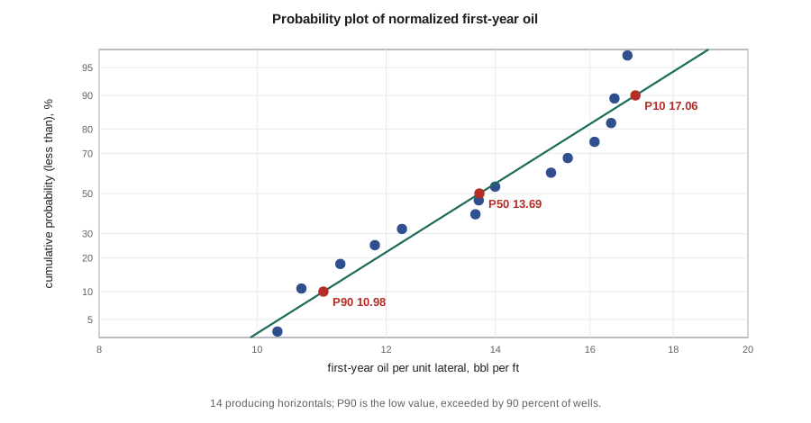
The normalized first-year volumes range from 10.3 to 16.9 barrels per foot of lateral. The lognormal fit gives a P90 of 11.0, a P50 of 13.7 and a P10 of 17.1 barrels per foot, a P10/P90 ratio of 1.55, which is narrow for a resource play and reflects consistent geology and completion practice. For a 9,800 foot lateral the P50 type well produces about 134,000 barrels in its first year and has an EUR of about 577,000 barrels; the P90 and P10 type wells have EURs of 463,000 and 719,000 barrels. The mean is only 1 percent above the P50 because the spread is small.

From type curves to undeveloped reserves

Each undeveloped location is assigned a type curve appropriate to its area and design. For the reserves categories, the question is what level of each type curve to use. A single well should not be booked at its median for proved reserves, because there is a 50 percent chance it will do worse. But a program of many wells has a much narrower range of total outcome than a single well, as Lesson 10 shows, so booking every well at its individual P90 would make the proved total for the program far too conservative. Practice varies; Graham's approach for the Phase 2 program is to use the P50 type curve for proved plus probable and a curve between the single-well P90 and P50, supported by a simulation of the program total, for proved.

The undeveloped forecast must also reflect timing and interference. Wells are scheduled according to the development plan, so their production starts in the year they are drilled, not at the effective date. Where new wells will be drilled close to existing ones, the forecasts for both should allow for interference, which can reduce the remaining reserves of the existing well and the EUR of the new one. The Bakken spacing pilot drilled two years ago showed about a 10 percent reduction in the EUR of wells drilled at the tightest spacing, and Graham applies that to the north flank locations.

Finally, type curves need to be revisited every year as new wells come on. A new well that performs well below the curve does not by itself prove the curve wrong, but a run of them is a strong signal, especially if they share a new completion design or a new area. Comparing actual results with the type curve each year, well by well and by vintage, is the best test of whether the evaluation is calibrated.