Decision trees, Monte Carlo and value of information

When Ethan presents the Spruce Ridge EMV, the exploration manager asks a question that EMV alone cannot answer. A seismic contractor has offered to shoot a small 3D survey over the structure for 0.6 million dollars before the well is drilled. Would that be money well spent? At the same meeting Diane asks how confident the company should be in the 5.92 million dollar value of a Phase 2 well, given everything that could go differently. This lesson covers the two tools that answer such questions: decision trees, which lay out sequences of decisions and uncertain events and identify the value of information, and Monte Carlo simulation of value, which turns uncertain inputs into a distribution of outcomes.

Decision trees

A decision tree is a diagram of a decision problem drawn from left to right in time order. Square nodes are decisions, where the company chooses a branch. Round nodes are chance events, where nature chooses a branch with stated probabilities. Each path ends in a terminal value, usually an NPV. The tree is solved by rolling back from right to left: at each chance node the value is the expected value of its branches, and at each decision node the value is that of the best branch. The result is both the value of the problem and the best strategy, including what to do after each possible outcome.

Trees force clarity. Drawing one requires stating every decision and uncertainty explicitly, in the order in which they occur, with probabilities that add to one at every chance node. That discipline alone often exposes muddled thinking, such as a plan that assumes a pilot will succeed before deciding whether to run it. Trees grow quickly, so practical ones are kept small and focused on the decisions that matter, with less important uncertainties handled by using expected values at the terminal nodes.

The value of information

Information has value only if it might change a decision. The expected value of perfect information is the most that any information about an uncertainty could be worth: it is the expected value if the company could learn the outcome before deciding, minus the expected value of the best decision without it. Real information is imperfect. A seismic survey can show whether the structure looks like a trap with a good seismic response, but a positive survey does not guarantee oil, and a negative one does not rule it out. The value of imperfect information is found by working out the revised probabilities after each possible survey result, using Bayes' theorem:

where S is success, D is dry, and + is a positive survey. The reliability of the information is described by two conditional probabilities: the chance of a positive survey if the prospect is truly a success, P(+|S), and the chance of a positive survey if it is dry, P(+|D), which is the false positive rate. These come from the geophysicists' experience with similar surveys in similar geology, and they should be estimated with the same honesty as Pg itself.

For Spruce Ridge, the geophysicists estimate that a 3D survey would show a positive response for 80 percent of real discoveries and for 25 percent of dry structures. The company would drill after a positive survey and walk away after a negative one, if the revised chance of success made drilling unattractive.

# Decision tree and value of information for 3D seismic over Spruce Ridge, then Monte Carlo on a Phase 2 well.
import random, math
SI = False     # True: Canadian case, False: US case
random.seed(11)
pg, win, dry, seis = (0.302, 22.0, 4.8, 0.6) if SI else (0.302, 18.0, 5.5, 0.6)   # millions
ev_now = max(0.0, pg * win - (1 - pg) * dry)
print(f"drill now: EV {pg * win - (1 - pg) * dry:.2f}; best without information {ev_now:.2f} million")
ev_perfect = pg * win                  # drill only when success is known
print(f"with perfect information EV {ev_perfect:.2f}; value of perfect information {ev_perfect - ev_now:.2f}")
pos_s, pos_d = 0.80, 0.25              # P(positive survey | success), P(positive survey | dry)
p_pos = pg * pos_s + (1 - pg) * pos_d
pg_pos = pg * pos_s / p_pos            # Bayes' theorem
pg_neg = pg * (1 - pos_s) / (1 - p_pos)
ev_pos = max(0.0, pg_pos * win - (1 - pg_pos) * dry)
ev_neg = max(0.0, pg_neg * win - (1 - pg_neg) * dry)
ev_info = p_pos * ev_pos + (1 - p_pos) * ev_neg
print(f"P(positive) {p_pos:.3f}; chance of success after positive {pg_pos:.3f}, after negative {pg_neg:.3f}")
print(f"EV after positive {ev_pos:.2f} (drill), after negative {ev_neg:.2f} ({'drill' if ev_neg > 0 else 'walk away'})")
print(f"value of imperfect information {ev_info - ev_now:.2f} vs survey cost {seis:.2f}: {'shoot the survey' if ev_info - ev_now > seis else 'skip the survey'}")
# Monte Carlo on one Phase 2 well, using the present values from Lesson 7 (millions)
pv_rev, pv_opex, cap0 = (13.67, 2.31, 5.2) if SI else (16.62, 3.69, 7.0)
npv = lambda e, p, c: pv_rev * e * p - pv_opex - cap0 * c     # e, p, c: multipliers on EUR, price and capital
res = []
for _ in range(20000):
    res.append(npv(math.exp(random.gauss(0, 0.35)), random.triangular(0.70, 1.30, 1.0), random.triangular(0.90, 1.25, 1.0)))
res.sort(); n = len(res)
print(f"Phase 2 well NPV10: P90 {res[int(0.1 * n)]:.2f}, P50 {res[n // 2]:.2f}, P10 {res[int(0.9 * n)]:.2f}, mean {sum(res) / n:.2f} million")
print(f"probability of a negative NPV {sum(r < 0 for r in res) / n:.1%}")
base = npv(1, 1, 1); z = 1.2816
for name, lo, hi in (("EUR (P90 to P10)", npv(math.exp(-z * .35), 1, 1), npv(math.exp(z * .35), 1, 1)),
                     ("price (-30 to +30 %)", npv(1, 0.7, 1), npv(1, 1.3, 1)),
                     ("capital (+25 to -10 %)", npv(1, 1, 1.25), npv(1, 1, 0.9))):
    print(f"tornado: {name:22s} {lo:6.2f} to {hi:6.2f} (swing {hi - lo:5.2f}; base {base:.2f})")

drill now: EV 1.60; best without information 1.60 million
with perfect information EV 5.44; value of perfect information 3.84
P(positive) 0.416; chance of success after positive 0.581, after negative 0.103
EV after positive 8.14 (drill), after negative 0.00 (walk away)
value of imperfect information 1.79 vs survey cost 0.60: shoot the survey
Phase 2 well NPV10: P90 -0.79, P50 5.49, P10 15.37, mean 6.57 million
probability of a negative NPV 14.3%
tornado: EUR (P90 to P10)        -0.08 to  15.34 (swing 15.42; base 5.93)
tornado: price (-30 to +30 %)     0.94 to  10.92 (swing  9.97; base 5.93)
tornado: capital (+25 to -10 %)   4.18 to   6.63 (swing  2.45; base 5.93)

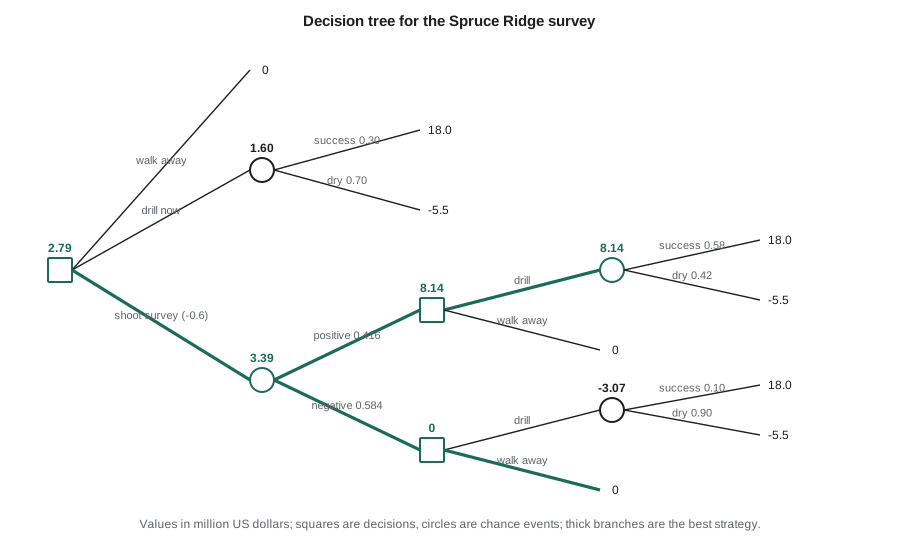
Drilling now has an expected value of about 1.6 million dollars. With perfect information the company would drill only successes, worth 5.44 million on average, so perfect information is worth 3.84 million: no survey, however good, could be worth more. With the actual survey, the chance of a positive result is 0.416. After a positive survey the chance of success rises from 0.30 to 0.58, and drilling is worth 8.1 million; after a negative survey it falls to 0.10, the well has a negative value, and the company walks away. The expected value with the survey is 1.79 million higher than drilling now, nearly three times its 0.6 million cost, so shooting the survey first is the better strategy.

The survey creates value by avoiding dry holes: in the negative case, which happens about 58 percent of the time, the company saves the cost of a well that would succeed only one time in ten. It also costs some value, because it delays the discovery and because about one real discovery in five will be missed after a misleading negative result. The calculation weighs these effects. Information about an outcome that would not change the decision is worth nothing: if the prospect were so good that the company would drill even after a negative survey, the survey would have no value.

Monte Carlo simulation of value

A decision tree handles a few discrete uncertainties well. When many continuous inputs are uncertain, as in the value of a development well, Monte Carlo simulation is more convenient. Each input is given a distribution, the cash flow model is run thousands of times with values sampled from those distributions, and the results form a distribution of NPV. The output answers questions a single number cannot: the probability that the well loses money, the range within which its value will probably fall, and which inputs drive the range.

For the Phase 2 well, Ethan uses three uncertain inputs: the EUR, lognormal with the spread of the type curve and its forecast uncertainty; the average oil price over the well's life, triangular from 70 to 130 percent of the deck; and the capital cost, triangular from 10 percent below to 25 percent above the estimate, because overruns are more common than savings. To keep the example short, the script uses the present values of revenue and operating cost from the Lesson 7 model and scales them with each sample.

The simulated NPV10 has a P90 of −0.79 million, a P50 of 5.49 million and a P10 of 15.4 million, with a mean of 6.57 million, higher than the deterministic 5.93 million because the lognormal EUR has a long upper tail. The probability of a negative NPV is about 14 percent. The mean, not the deterministic value, is what a program of such wells will deliver on average, which is one reason simulation is worth doing even when the deterministic answer is positive.

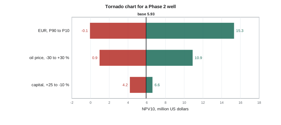
The tornado chart ranks the inputs by their effect when each is moved across its range with the others held at their base values. EUR has the largest swing, followed by price; capital has a much smaller effect. The chart tells the company where better information would be most valuable: here, in narrowing the EUR forecast through more production data, better type curves or early-time diagnostics, rather than in refining the cost estimate.

Using probabilistic results well

Monte Carlo results look precise, and that is their main danger. The output is only as good as the input distributions and the dependencies between them. Ranges that are too narrow, which is the usual failing, produce outputs that are too narrow. Ignoring correlation, for example between oil price and service costs, which tend to rise and fall together, distorts the tails. A simulation run should therefore always be accompanied by a short statement of the input ranges and their basis, so that reviewers can challenge them.

Simulation and decision trees also work together. A tree's terminal values can be the means of simulated distributions, and a simulation can include decisions, such as stopping development if early wells disappoint, which captures the value of flexibility. The aim is not mathematical sophistication but better decisions: knowing which uncertainties matter, what information would resolve them, and how much that information is worth.

Ethan presents the two results together. The survey decision is clear: the information is worth about twice its cost or more, so the exploration team should shoot it before committing to the well, and the 2027 budget should carry the well as conditional on a positive result. The Phase 2 simulation supports drilling the remaining wells but changes how the results are reported to the board: rather than a single value per well, the board sees the P90 to P10 range and the probability of a loss, and understands that a disappointing first well would not by itself mean the program had failed.