Decline curve analysis

Most of the company's proved developed producing reserves come from wells that have produced long enough to show a trend. For those wells the standard method is decline curve analysis: fitting an empirical curve to the production history and extending it to the economic limit. Ethan's first assignment is the 3-22H well, the first Bakken horizontal in the field, which now has 30 months of history. Graham warns him that the method looks simple and is easy to abuse. “Any curve fits two years of data. The question is whether the curve you pick will still be right in year fifteen, and that depends on understanding why the well is declining.”

Decline rate and the Arps equations

The instantaneous decline rate is the fractional rate at which production falls:

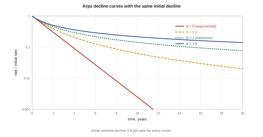
In 1945 J. J. Arps proposed a family of curves in which the decline rate itself changes with rate as D = K q^b, where b is a constant. Integrating gives the three classic forms. When b = 0 the decline rate is constant and the decline is exponential. When b = 1 the decline is harmonic. For values of b between these, and above them, the decline is hyperbolic:

where q_i is the rate at the start of the fitted period and D_i is the initial nominal decline rate. The cumulative production follows directly. For exponential decline the cumulative to rate q is (q_i − q)/D, and for hyperbolic decline with b not equal to 1 it is

Decline rates can be stated as nominal rates, the D of the equations, or as effective rates, the fractional drop in rate over one year. For exponential decline the effective annual decline is 1 − e^(−D), so a nominal rate of 0.20 per year is an effective decline of 18.1 percent. Reports and software use both, so the convention must always be stated.

What b means physically

The Arps equations were empirical, but later work tied the exponent to the flow regime. A well producing a closed reservoir at constant bottomhole pressure in boundary-dominated flow declines with b between 0 and about 0.5: near 0 for single-phase liquid, around 0.3 for solution-gas drive as gas saturation builds, and up to about 0.5 for gas wells and some water-drive systems. Values above 1 cannot persist in boundary-dominated flow, because they imply infinite cumulative production.

Multi-stage fractured horizontal wells in tight rock behave differently. For months or years they are in transient linear flow from the matrix into the fractures, which on a log-log plot of rate against time appears as a straight line of slope −1/2. Fitting an Arps curve to transient linear flow gives b close to 2, and fits to early unconventional data commonly give b between 1 and 2. When the pressure disturbance reaches the boundaries of the drainage volume, typically halfway to the neighboring well, the decline steepens toward boundary-dominated behavior. Extending a high-b curve indefinitely therefore overstates the reserves, sometimes by a large factor.

The modified hyperbolic decline

The common practical answer is the modified hyperbolic decline: a hyperbolic curve with the fitted b until its decline rate falls to a chosen terminal value, then an exponential decline at that terminal rate. Because the nominal decline of a hyperbolic curve is D(t) = D_i/(1 + b D_i t), the switch happens when D(t) equals the terminal nominal rate D_min, at a time

Terminal decline rates between 5 and 10 percent per year effective are typical for tight oil; the evaluator should support the value with analogs, older wells in the same play, or rate-transient analysis that estimates when boundary effects begin. Choosing the terminal rate is one of the most consequential judgments in an unconventional evaluation, because the late-life tail can contain a third or more of a well's reserves.

Fitting the 3-22H well

Before fitting, the data must be cleaned. Monthly volumes should be converted to rates on a producing-day basis so that downtime does not look like decline. Months affected by workovers, artificial lift changes, offset frac interference or shut-ins for facility work should be flagged and either excluded or explained. Rate changes from choke adjustments in the first months are not reservoir decline. Ethan also plots rate against cumulative production, which straightens exponential decline and is less sensitive to downtime, and a log-log rate-time plot to identify the flow regime.

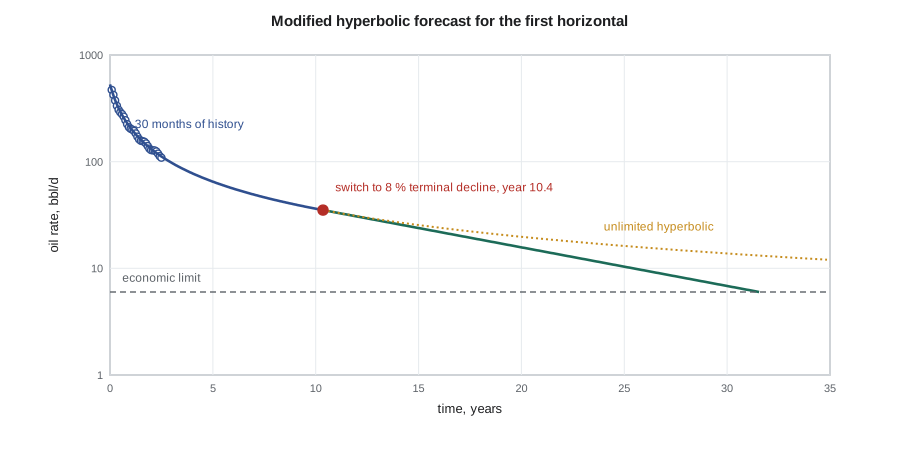
The script below fits a hyperbolic curve to the 30 months of cleaned history by least squares on the logarithm of rate, applies an 8 percent effective terminal decline, and extends the forecast to an economic limit of 6 bbl/d.

# Arps decline: fit a hyperbolic curve to monthly rates, switch to a terminal exponential decline, and compute EUR.
import math
SI = False     # True: m3/d, False: bbl/d
# synthetic history for the first horizontal: 30 months of daily-average rates (illustrative)
qi_t, Di_t, b_t = (38.0, 1.6, 1.1) if SI else (520.0, 1.6, 1.1)    # rate, nominal 1/yr, b
hist = [qi_t / (1 + b_t * Di_t * (m / 12)) ** (1 / b_t) * (1 + 0.03 * math.sin(m)) for m in range(1, 31)]
def arps(t, qi, Di, b):                                           # t in years
    return qi * math.exp(-Di * t) if b == 0 else qi / (1 + b * Di * t) ** (1 / b)
best = None
for qi in [qi_t * (0.85 + 0.01 * i) for i in range(31)]:
    for Di in [0.8 + 0.05 * j for j in range(33)]:
        for b in [0.5 + 0.1 * k for k in range(12)]:
            e = sum((math.log(arps(m / 12, qi, Di, b)) - math.log(q)) ** 2 for m, q in enumerate(hist, 1))
            if best is None or e < best[0]: best = (e, qi, Di, b)
_, qi, Di, b = best
unit = "m3/d" if SI else "bbl/d"; vol = "m3" if SI else "bbl"
print(f"fitted qi {qi:.1f} {unit}, Di {Di:.2f} per year (nominal), b {b:.1f}")
Dterm = -math.log(1 - 0.08)                      # terminal decline: 8 percent per year effective
t_sw = (Di / Dterm - 1) / (b * Di)               # time when the hyperbolic nominal decline falls to Dterm
q_sw = arps(t_sw, qi, Di, b)
qlim = 1.0 if SI else 6.0                        # economic limit rate
def cum_to(t):                                   # cumulative to time t (years) under the modified hyperbolic
    days = 365.25
    if t <= t_sw:
        return days * qi / ((1 - b) * Di) * (1 - (arps(t, qi, Di, b) / qi) ** (1 - b))
    Np_sw = cum_to(t_sw)
    return Np_sw + days * q_sw / Dterm * (1 - math.exp(-Dterm * (t - t_sw)))
t_lim = t_sw + math.log(q_sw / qlim) / Dterm
print(f"switch to terminal decline after {t_sw:.1f} years at {q_sw:.1f} {unit}")
print(f"economic limit {qlim} {unit} reached after {t_lim:.1f} years")
print(f"EUR (modified hyperbolic) {cum_to(t_lim):,.0f} {vol}; first-year volume {cum_to(1.0):,.0f} {vol}, EUR / first year {cum_to(t_lim) / cum_to(1.0):.1f}")
pure = 365.25 * qi / ((1 - b) * Di) * (1 - (qlim / qi) ** (1 - b))
print(f"EUR if the b = {b:.1f} curve were never limited {pure:,.0f} {vol}  (+{100 * (pure / cum_to(t_lim) - 1):.0f} percent)")
for name, bb in (("exponential", 0.0), ("harmonic", 1.0)):
    if bb == 0: eur = 365.25 * (qi - qlim) / Di
    else: eur = 365.25 * qi / Di * math.log(qi / qlim)
    print(f"EUR with the same qi and Di, {name:11s} {eur:,.0f} {vol}")

fitted qi 530.4 bbl/d, Di 1.65 per year (nominal), b 1.1
switch to terminal decline after 10.4 years at 35.2 bbl/d
economic limit 6.0 bbl/d reached after 31.6 years
EUR (modified hyperbolic) 493,780 bbl; first-year volume 115,833 bbl, EUR / first year 4.3
EUR if the b = 1.1 curve were never limited 663,928 bbl  (+34 percent)
EUR with the same qi and Di, exponential 116,083 bbl
EUR with the same qi and Di, harmonic    526,222 bbl

The fit gives an initial rate of 530 bbl/d, an initial nominal decline of 1.65 per year and b = 1.1. The decline reaches the terminal rate after 10.4 years, when the well makes about 35 bbl/d, and the economic limit is reached after about 32 years. The estimated ultimate recovery (EUR), including the volume already produced, is about 494,000 barrels, 4.3 times the first-year volume. Leaving the b = 1.1 curve unlimited would add 34 percent; forcing an exponential decline with the same initial decline would cut the EUR by three quarters, which shows that the choice of model, not the fit statistics, controls the answer.

From one forecast to reserves categories

A decline forecast is a single line, but reserves need a range. For producing wells the range comes from the uncertainty in b, the terminal decline and the timing of boundary effects, and sometimes from the possibility of interference from future offset wells. Graham's practice for the Bakken horizontals is to use the best-fit curve with the 8 percent terminal decline for the proved plus probable case, a lower b and a 10 percent terminal decline for proved, and a higher b with a 6 percent terminal decline for proved plus probable plus possible. He checks that the proved forecasts for the group of producing wells add up to a total that the wells have a high chance of exceeding.

Producing-well forecasts should also be checked against physical limits and analogs. The EUR should be plausible relative to the oil in place in the well's drainage area, typically a recovery factor of 5 to 15 percent for tight oil. The forecast should be consistent with older wells in the play that are further along in their decline. And the economic limit should come from the actual operating costs of the well or its battery, not from a rule of thumb. Lesson 7 shows how the cash flow sets the economic limit directly.

Other decline models

Several alternatives to Arps have been proposed for unconventional wells. The power-law exponential and stretched exponential models add a time-varying decline that tends naturally toward a lower late-time rate. Duong's model is built on the linear flow regime and fits fracture-dominated flow well, but it can overstate late-time rates if boundary effects are not added. Rate-transient analysis, which uses both rate and flowing pressure and fits analytical flow models, can estimate the effective fracture area and the time to boundary-dominated flow, and so gives a physical basis for the terminal decline. Whatever model is used, the evaluator must explain why it suits the well and test the forecast against analogs; regulators and auditors accept many methods but not unexplained ones.

Ethan finishes the producing-well forecasts by grouping the wells and looking at them together. Plotting all 14 horizontals normalized by lateral length on one chart shows immediately which wells are outliers, and comparing each well's fitted b and terminal decline with its neighbors catches fits that are statistically good but physically odd. Two older wells stand out: their recent rates have fallen faster than the hyperbolic fits predicted, a sign that they have reached boundary-dominated flow earlier than the others. Graham agrees to switch them to terminal decline now, which becomes the downward technical revision in the year-end reconciliation of Lesson 12.