Pipelines, compression and LNG

Residue gas leaves the Ten Mile Ridge processing plant at about 650 psia. To reach the sales point at the Dominion South hub it must travel about 42 miles by pipeline and arrive above the transmission system's receipt pressure of about 800 psia. Sofia owns the sales line design, and she asks Ethan to work through the flow equations with her. “The reservoir decides how much gas you have,” she says. “The pipeline decides how much you can sell on a cold day in January, when every customer wants it.” This lesson covers steady-state gas pipeline flow, design pressure under 49 CFR Part 192, compression, and the LNG export chain that now pulls on gas from both the Marcellus and its neighbors.

The general flow equation

Gas flowing in a pipeline loses pressure to friction, and because it expands as pressure falls, its velocity rises along the line. A steady-state energy balance for isothermal flow in a horizontal pipe, neglecting the small kinetic energy change, gives the general flow equation. In US customary units, with q_sc in scf/d, base temperature T_b in °R and base pressure p_b in psia, D the inside diameter in inches, L the length in miles, T_f the flowing temperature and z̄ the average z-factor:

The Fanning friction factor f, or its Darcy equivalent, depends on the Reynolds number and the pipe roughness. Because gas pipelines run at high Reynolds numbers, most flow is either partially turbulent, where f depends on the Reynolds number, or fully turbulent, where it depends only on roughness. The pressure-squared difference appears for the same reason as in the well inflow equation: the gas expands as it flows.

Before computers, engineers replaced the friction factor with simple correlations, giving the classic pipeline equations still found in tariffs and design manuals. The Weymouth equation (1912) uses f proportional to D^(−1/3) and is conservative for large-diameter, high-flow lines. The Panhandle A (1940s) and Panhandle B (1956) equations use friction factors that fall with Reynolds number and suit long transmission lines in partially turbulent flow. The AGA fully turbulent equation and the Colebrook-White equation solved iteratively are used for detailed design. A pipeline efficiency factor E, typically 0.90 to 0.95, absorbs bends, fittings, deposits and the difference between ideal and real pipe.

That is Panhandle B in US customary units, with q_sc in scf/d. Elevation changes add a hydrostatic term, important in hilly terrain such as the Appalachians or the foothills of the Rockies. Because pressure-squared falls linearly with distance in a uniform line, the pressure itself falls more steeply near the outlet, where the gas is less dense and moves faster.

# Sales pipeline from the plant: Weymouth and Panhandle B capacities, design pressure from Barlow's formula,
# and the compressor power to boost residue gas from plant outlet to pipeline pressure.
import math
SI = False     # True: metric units, False: oilfield units

gg, T_R, Z = 0.62, 60 + 459.67, 0.90           # residue gas gravity, flowing temperature, average z
Tb, pb = 520.0, 14.73                          # base conditions, deg R and psia
L_mi, D_in, E = 42.0, 19.25, 0.95               # length (miles), inside diameter (in), pipeline efficiency
p1, p2 = 1300.0, 800.0                          # inlet and outlet pressure, psia

def weymouth(p1, p2):
    return 433.5 * E * (Tb / pb) * ((p1 ** 2 - p2 ** 2) / (gg * T_R * L_mi * Z)) ** 0.5 * D_in ** 2.667 / 1e6

def panhandle_b(p1, p2):
    return 737.0 * E * (Tb / pb) ** 1.02 * ((p1 ** 2 - p2 ** 2) / (gg ** 0.961 * T_R * L_mi * Z)) ** 0.51 * D_in ** 2.53 / 1e6

qw, qp = weymouth(p1, p2), panhandle_b(p1, p2)
cv = 0.0283168                                  # 10^6 m3 per MMscf
print(f"Weymouth {qw * cv:.2f} x 10^6 m3/d, Panhandle B {qp * cv:.2f} x 10^6 m3/d" if SI else
      f"Weymouth {qw:,.0f} MMscf/d, Panhandle B {qp:,.0f} MMscf/d")
# pressure along the line at the Panhandle B rate: p(x)^2 = p1^2 - (p1^2 - p2^2) x / L
for frac in (0.0, 0.25, 0.5, 0.75, 1.0):
    p = math.sqrt(p1 ** 2 - (p1 ** 2 - p2 ** 2) * frac)
    print(f"  {frac * L_mi * 1.609:5.1f} km  {p / 0.145038:6,.0f} kPa" if SI else f"  {frac * L_mi:5.1f} mi  {p:6,.0f} psia")

# Barlow design pressure, NPS 20 pipe: OD 20 in, wall 0.375 in, grade X70 (SMYS 70,000 psi)
OD, t, S = 20.0, 0.375, 70000.0
F = 0.72 if not SI else 0.80                     # design factor: Class 1 under 49 CFR 192 / Class 1 under CSA Z662
P = 2 * S * t / OD * F                          # psig (joint and temperature factors 1.0)
print(f"Design pressure {P * 6.894757:,.0f} kPa with design factor {F:.2f} (CSA Z662 Class 1)" if SI else
      f"Design pressure {P:,.0f} psig with design factor {F:.2f} (49 CFR 192 Class 1)")

# Compressor: residue gas 125 MMscf/d from plant outlet 650 psia to 1,300 psia in two stages with intercooling to 80 F
k, Ts, eff, ps, pd, Zs = 1.28, 540.0, 0.78, 650.0, 1300.0, 0.92
q = 125e6                                       # scf/d of residue gas
r = (pd / ps) ** 0.5                            # equal ratio per stage
n = q / 379.5 / 86400                           # lb-mol/s
head = k / (k - 1) * Zs * 1545.35 * Ts * (r ** ((k - 1) / k) - 1)   # ft.lbf per lb-mol, adiabatic
hp = 2 * n * head / 550 / eff
Td = Ts * (1 + (r ** ((k - 1) / k) - 1) / eff) - 459.67
print(f"Ratio per stage {r:.2f}; discharge {(Td - 32) / 1.8:.0f} C before cooling; compressor power about {hp * 0.7457:,.0f} kW" if SI else
      f"Ratio per stage {r:.2f}; discharge {Td:.0f} F before cooling; compressor power about {hp:,.0f} hp")

Weymouth 360 MMscf/d, Panhandle B 453 MMscf/d
    0.0 mi   1,300 psia
   10.5 mi   1,195 psia
   21.0 mi   1,079 psia
   31.5 mi     950 psia
   42.0 mi     800 psia
Design pressure 1,890 psig with design factor 0.72 (49 CFR 192 Class 1)
Ratio per stage 1.41; discharge 135 F before cooling; compressor power about 4,913 hp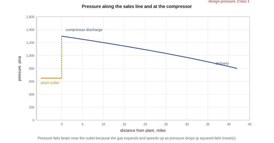

With an NPS 20 line, 19.25 inches inside diameter, a discharge pressure of 1,300 psia and a delivery pressure of 800 psia, Panhandle B gives a capacity of about 450 MMscf/d and Weymouth, the conservative choice, about 360 MMscf/d. Both far exceed the plant's initial 125 MMscf/d of residue gas. Sofia explains the reasoning: pipe is cheap to oversize at construction and very expensive to loop later, and Prairie Crest expects to expand the plant or bring third-party gas into the line. At the initial throughput the line could run at a lower inlet pressure, saving compression.

Design pressure and pipeline codes

The wall thickness of a gas pipeline is set by Barlow's formula for hoop stress, with a design factor that depends on the population near the line. In the United States, gas transmission and many gathering lines are regulated by PHMSA under 49 CFR Part 192. The design pressure is P = (2St/D) × F × E × T, where S is the specified minimum yield strength, t the wall thickness, D the outside diameter, F a design factor of 0.72 in Class 1 locations falling to 0.40 in Class 4, E the longitudinal joint factor and T the temperature derating factor. A 2021 PHMSA rule extended safety requirements to many previously unregulated rural gathering lines, defined as Type C, and later rules added requirements for rupture-mitigation valves and integrity management. For the NPS 20 line with 0.375-inch wall in grade X70 steel, the design pressure is about 1,890 psig, well above the planned operating pressure.

Class location matters as much as the formula. As houses are built near a line over its life, its class location can change, lowering the allowed operating pressure unless the pipe is replaced or tested. Pipeline integrity management, with in-line inspection by smart pigs, cathodic protection, coating surveys, leak detection and damage prevention programs, keeps the line safe through its decades of service. The Ten Mile Ridge line's route avoids the few homes in the area and will be built for in-line inspection from the start.

Compression

Compressors raise gas pressure at the plant inlet when the field pressure falls, at the plant outlet to reach the sales line, and along transmission lines every 50 to 100 miles. Reciprocating compressors, driven by gas engines or electric motors, handle high ratios and variable conditions and dominate field and plant service. Centrifugal compressors, driven by gas turbines or motors, handle large volumes at modest ratios and dominate transmission. The power for adiabatic compression of a real gas from suction pressure p_s to discharge pressure p_d is:

per mole of gas, divided by the adiabatic efficiency, typically 0.75 to 0.85. Here k is the ratio of specific heats, about 1.25 to 1.3 for natural gas. The discharge temperature rises with the compression ratio, and practical limits on temperature and rod load keep reciprocating stages to ratios of about 3 to 4. Higher overall ratios use several stages with intercoolers between them, and equal ratios per stage minimize total power. For the Ten Mile Ridge processing plant's sales compressor, a two-stage machine with a ratio of about 1.4 per stage needs roughly 4,900 hp to move 125 MMscf/d, close to the rule of thumb of 40 hp per MMscf/d for an overall ratio of 2. Compressor fuel or electricity is one of the largest operating costs of a gas system, and electrifying compression, using power from the grid rather than gas engines, cuts emissions where clean grid power is available, as it is in much of Pennsylvania.

LNG: the export link

Liquefied natural gas connects North American gas to world markets. Gas is treated to remove carbon dioxide, water, mercury and heavy hydrocarbons, then cooled to about −162 °C in large refrigeration trains, at which point it condenses to a liquid about 1/600 of its gaseous volume. The liquid is stored in insulated tanks, loaded onto LNG carriers and regasified at the receiving terminal. Liquefaction uses roughly 8 to 12 percent of the feed gas as fuel, unless the trains are driven electrically.

The United States is the world's largest LNG exporter. Exports grew rapidly in 2025 as new capacity such as Plaquemines LNG in Louisiana ramped up, with monthly exports setting records. US marketed gas production reached a record of about 118.5 Bcf/d in 2025, according to the EIA, and the Appalachian Basin, led by the Marcellus, supplied about 31 percent of it. Most export terminals are on the Gulf Coast, closer to the Haynesville and Permian than to Appalachia, so Marcellus gas reaches LNG markets mostly by displacement and through pipelines to the south and east, and pipeline capacity out of the basin is a recurring constraint on prices at hubs such as Dominion South.

For the Ten Mile Ridge plan, the LNG link matters through price and access. Gas sold at the Dominion South hub takes the regional price, which often trades at a discount to Henry Hub when pipelines out of the basin are full; new takeaway capacity and LNG-driven demand along the Atlantic and Gulf coasts narrow that discount. Lesson 12 uses a planning price that reflects these factors.