
PET-440 · Lesson 12 of 12 · 20 min
Capstone: a gas field development plan
Eight months after the acquisition, Lena asks the Ten Mile Ridge team for a development plan she can take to the board: how many wells, how fast, what plant, what pipeline, what it costs, what it earns and what could go wrong. Farid assigns the pieces. Ethan builds the production forecast and the economics from the type well; Sofia and Gwen own the plant and pipeline; Mei confirms the fluid and product specifications; Farid reviews the reserves and the risks. “A development plan is a set of linked decisions,” Farid tells Ethan. “The plant size sets the drilling pace, the drilling pace sets the capital curve, and the capital curve sets whether the project is worth doing at all.” This lesson walks through the plan and the reasoning behind each choice, using the tools of Lessons 1 to 11.
Step 1: the resource and the type well
The plan starts with the resource. The Ten Mile Ridge block covers about 48 square miles of Marcellus rights in which the team has mapped one landing zone with consistent thickness, pressure and liquids yield. Volumetrics from Lesson 3 give about 61 Bscf of free gas per spacing unit in that zone, about 20 percent more adsorbed gas from Lesson 8, and about 2.6 million barrels of condensate per spacing unit from Lesson 7. The type well, calibrated by rate-transient analysis of the four existing wells, starts at 8 MMscf/d and has a 30-year EUR of about 7.4 Bscf of raw gas. At four wells per spacing unit, it recovers roughly half of the free gas in the landing zone; the spacing pilots will test that assumption.
Reserves follow the SEC rules and SPE-PRMS. Before sanction, the existing four wells and their direct offsets can carry proved and probable reserves; the rest of the program is contingent resource until the project is approved and funded, when undeveloped locations within reasonable distance of producing wells can be booked as proved undeveloped. Farid insists that the type well used for the plan be the P50 of the existing wells' range, with P90 and P10 type wells for the sensitivities, rather than the best well.
Step 2: plant size and drilling pace
The team considers plant sizes of 100, 150 and 200 MMscf/d. A bigger plant has lower unit cost and brings more gas forward, but needs more wells per year to fill and keep full, a bigger rig and frac fleet commitment and more capital before first gas. The pipeline of Lesson 11 can carry any of them. The middle option, 150 MMscf/d of raw gas, matches the drilling capacity Prairie Crest can commit, one drilling rig and a shared completion crew delivering about 14 wells per year, and the gas sales commitments marketing expects to sign.
# Field development plan: wells needed to fill a 150 MMscf/d (4.25 x 10^6 m3/d) plant with the Lesson 8 type well,
# the resulting production profile, and a simple before-tax NPV at 10 percent.
import math
SI = False     # True: Canadian case (CAD, royalty, AECO-style price), False: US case (USD, Dominion South-style price)

qi, Di, b, Dterm = 8.0, 1.5, 1.0, 0.06           # type well from Lesson 8 (MMscf/d, 1/yr)
Dlim = -math.log(1 - Dterm); t_sw = (Di / Dlim - 1) / (b * Di)
def rate(t):                                      # MMscf/d at time t (years) after first production
    if t < 0: return 0.0
    if t < t_sw: return qi / (1 + b * Di * t) ** (1 / b)
    return qi / (1 + b * Di * t_sw) ** (1 / b) * math.exp(-Dlim * (t - t_sw))
def avg(t0):                                      # average rate in the year starting at t0 (12 monthly steps)
    return sum(rate(t0 + (m + 0.5) / 12) for m in range(12)) / 12

plateau, years, max_wells = 150.0, 20, 14
starts = []                                       # each well starts on its year's first day
for y in range(years):
    n = 0
    while n < max_wells and sum(avg(y - s) for s in starts) + n * avg(0) < plateau * 0.98: n += 1
    starts += [y] * n
prod = [min(plateau, sum(avg(y - s) for s in starts)) for y in range(years)]
wells = [starts.count(y) for y in range(years)]

price = 3.10 if SI else 3.30                      # gas price per Mscf at the plant gate after transport (dollars)
liq = 1.10 if SI else 0.70                        # NGL and condensate uplift, dollars per Mscf of raw gas
roy = 0.12 if SI else 0.15                        # effective royalty on revenue
opex, plant_cost = 0.75, 260e6                   # dollars per Mscf; dollars for the plant and gathering
well_cost = 7.5e6 if SI else 8.0e6               # dollars per well, drilled and completed
# Year 0: build the plant and drill the first wells; each later well is drilled the year before it starts.
npv = cum = 0.0
cf0 = -plant_cost - wells[0] * well_cost
npv += cf0 / 1.1 ** 0.5; cum += cf0
print("year wells  raw gas  net cash flow" + ("  (10^6 m3/d, million CAD)" if SI else "  (MMscf/d, million USD)"))
print(f"   0 {wells[0]:5d}     0.00  {cf0 / 1e6:10.1f}")
for y in range(1, years + 1):
    vol = prod[y - 1] * 365 * 1e3                 # Mscf produced in the year
    nxt = wells[y] if y < years else 0            # wells drilled this year for next year
    cf = vol * ((price + liq) * (1 - roy) - opex) - nxt * well_cost
    npv += cf / 1.1 ** (y + 0.5); cum += cf
    if y < 6 or y % 5 == 0:
        g = prod[y - 1] * 0.0283168 if SI else prod[y - 1]
        print(f"{y:4d} {nxt:5d}  {g:7.2f}  {cf / 1e6:10.1f}" if SI else f"{y:4d} {nxt:5d}  {g:7.1f}  {cf / 1e6:10.1f}")
plateau_years = sum(1 for p in prod if p >= plateau * 0.97)
print(f"Wells drilled {len(starts)}; plateau held about {plateau_years} years; NPV10 {npv / 1e6:,.0f} million; undiscounted {cum / 1e6:,.0f} million")year wells raw gas net cash flow (MMscf/d, million USD) 0 14 0.00 -372.0 1 14 68.4 -45.9 2 14 103.5 -11.9 3 14 127.2 11.1 4 12 145.2 44.5 5 10 150.0 65.1 10 8 150.0 81.1 15 8 150.0 81.1 20 0 149.4 144.5 Wells drilled 192; plateau held about 16 years; NPV10 25 million; undiscounted 937 million
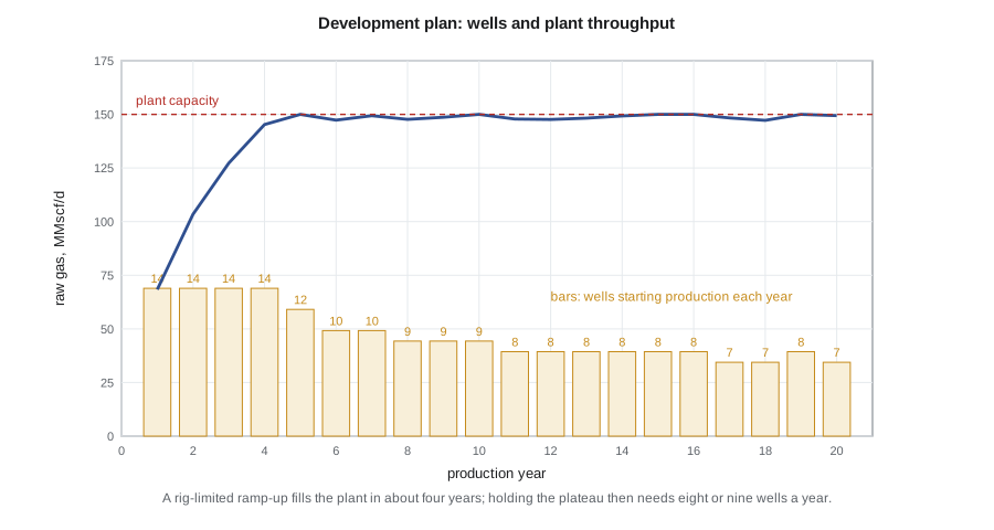
The forecast shows the treadmill typical of tight gas. With 14 wells starting in each of the first four years, the plant fills in year 5. From then on, because each well loses roughly 60 percent of its rate in its first year, eight or nine new wells are needed every year just to hold the plateau. Over 20 years the plan drills about 190 wells, nearly the whole block at four wells per spacing unit. If the type well proves 20 percent better than the base case, about 30 fewer wells are needed; if it is 20 percent worse, about 40 more, and the block's inventory would run short before year 20.
Step 3: economics
The economic model is deliberately simple at this stage: before tax, real terms, with a gas price at the plant gate after transportation, a liquids uplift per unit of raw gas from the condensate and NGL sales, a royalty, an operating cost per unit, a well cost and the plant and gathering capital. The base case uses USD 3.30 per thousand cubic feet of raw gas at the plant gate, reflecting a discount to Henry Hub at the Dominion South hub, a liquids uplift of USD 0.70, a landowner royalty of 15 percent, operating costs of USD 0.75, wells at USD 8.0 million and a plant and gathering system at USD 260 million. Taxes, inflation and abandonment costs are left for the detailed model.
The base case gives an NPV at 10 percent of about USD 25 million and undiscounted net cash flow of about USD 0.9 billion. The project pays out in about year 10. The large early capital, USD 372 million in year 0 for the plant and the first wells, and the continuing drilling capital are characteristic of tight gas: the field never stops being a capital project.
| Case (one factor changed) | NPV10, million USD |
|---|---|
| Base case | 25 |
| Gas price +20 percent | 247 |
| Gas price −20 percent | −197 |
| Type well +20 percent | 172 |
| Type well −20 percent | −179 |
| Well cost −20 percent | 180 |
| Well cost +20 percent | −130 |
| Plant cost +30 percent | −50 |
The sensitivities tell the story. Gas price and type-well performance each move the NPV by more than its base value for a 20 percent change, and the project loses money at the low end of either. Well cost matters more than plant cost, because about 190 wells are drilled against one plant. The US case is marginal at the base price; it works only with a higher regional price, better wells or lower well costs, which is why the plan's first phase is designed to prove those.
Worked problem
Payout and capital efficiency
The base case spends USD 372 million in year 0 and has net cash flows in years 1 to 6 of −45.9, −11.9, 11.1, 44.5, 65.1 and 62.5 million, and about USD 70 million a year after that. When does cumulative cash flow turn positive, and what is the capital efficiency, the NPV divided by the discounted capital?
Show solution
- Cumulative after year 0: −372. After year 1: −417.9. After year 2: −429.8.
- After year 3: −418.7. After year 4: −374.2. After year 5: −309.1. After year 6: −246.6.
- Two more years at about USD 71 million leave −103.3 after year 8; with year 9 at 71.8 and year 10 at 81.1, cumulative cash turns positive in year 10.
- Discounted capital, plant plus all wells, is roughly USD 1.02 billion, so capital efficiency is 25 / 1,020 = 0.02.
Answer: Payout takes about ten years with continuous drilling, and each discounted dollar of capital returns about 2 cents of NPV. A better phase-one result, from longer laterals, better targeting or lower costs, would shorten payout sharply.
Step 4: facilities, market and regulatory plan
The plant and pipeline design follows Lessons 9 to 11. The Ten Mile Ridge processing plant includes inlet separation and condensate stabilization, TEG and molecular sieve dehydration, a turboexpander with flexible ethane recovery or rejection and sales compression into an NPS 20 line to the Dominion South hub; no amine unit is needed for pipeline-quality gas. The gathering system uses wet gas lines with methanol injection in winter, and pad separators with free-water knockout. Electric drive is chosen for the sales compressors where the grid connection allows, cutting fuel use and emissions.
The regulatory plan lists the approvals and their timing: well permits from the DEP under the state's oil and gas regulations, erosion and sediment control and water management plans, air quality permits for the plant, PHMSA and state requirements for the gathering lines and the sales pipeline, federal methane emission rules, and road-use and community agreements with the townships along the pipeline route. Each has a lead time that the schedule must respect.
Step 5: risks and the phased decision
Farid's risk register lists the uncertainties that could change the decision. Subsurface: type-well performance and its variation across the block, the effect of well spacing and parent-child interference, condensate banking in the near-fracture region, and the liquids yield away from the existing wells. Commercial: gas and liquids prices, regional price differentials and pipeline access. Execution: well cost inflation, rig and frac crew availability, and plant cost and schedule. Regulatory and social: permitting timelines, water supply, induced seismicity and community acceptance. Emissions: methane intensity and its reporting, which buyers, especially LNG customers, increasingly demand.
The team's recommendation is a phased plan. Phase 1, over 18 months, drills two spacing-pilot pads, runs the managed-drawdown comparison from Lesson 7, tests the disposal well and signs the gas, condensate and NGL contracts. At the end of phase 1, the board decides on the full plant with the type well and costs re-estimated from the pilots. Meanwhile, the existing four wells and the Oriskany sandstone pool keep producing through the third-party plant, generating cash and data. Ethan writes the summary for the board in a single page: what is known, what is not, what phase 1 will learn, and what it costs to learn it. Farid reads it and nods. “That,” he says, “is a development plan.”
Looking back at the course
Every step of the plan used the tools of this course. The composition and phase behavior set the fluid type and the processing. The z-factor and gas properties turned pressures into volumes. Volumetrics and material balance estimated the gas in place and checked it against production, and the water influx and overpressure corrections kept the estimates honest. Deliverability and well tests described how the wells produce and what limits them. The condensate lesson priced the liquids and the losses. The tight gas lesson built the type well that drives everything. Dehydration, hydrate control, treating and NGL recovery turned raw gas into sellable products, and the pipeline, compression and LNG lessons connected the field to its market. The economics brought them together into a decision.
Common mistakes
MistakeUsing the best existing well as the type well.
InsteadUse the P50 of the range, with P90 and P10 cases for sensitivity, calibrated to all available wells.
MistakeSizing the plant without checking the drilling pace needed to fill and hold it.
InsteadModel wells per year against rig and crew capacity and the inventory of locations.
MistakeTreating the plant as the main capital and the wells as an afterthought.
InsteadIn tight gas, continuous drilling dominates capital and sensitivity.
MistakeCommitting to full development before testing the key uncertainties.
InsteadPhase the decision: spend modestly to learn about spacing, well performance and costs first.
Summary and key terms
- A gas development plan links resource, type well, plant size, drilling pace, facilities, market and economics.
- Tight gas plateau requires continuous drilling because each well declines steeply in its first year.
- Gas price, type-well performance and well cost dominate the economics; plant cost matters less.
- Reserves booking follows the SEC rules and SPE-PRMS; undeveloped locations become reserves when the project is sanctioned and funded.
- Regulatory approvals, community agreements and emissions requirements set the schedule as much as engineering does.
- A phased plan that tests the key uncertainties before full commitment is the usual way to manage risk.
- Development plan
- An integrated plan of wells, facilities, schedule, costs and economics for a field.
- Plateau
- The period during which production is held at facility capacity.
- Payout
- The time at which cumulative net cash flow becomes positive.
- Capital efficiency
- NPV divided by discounted capital investment.
- Sensitivity analysis
- Testing how results change when one input is varied at a time.
- Phased development
- Staging investment decisions to learn about key uncertainties before committing fully.
Practice problems
Work each problem on paper first, then reveal the answer to check.
Why does the plan need eight or nine new wells a year once the plant is full?
Show answer
Each well's rate falls by more than half in its first year, so new wells must replace that decline.
Which single factor in the sensitivity table matters most for the US case?
Show answer
Gas price and type-well performance, which each swing the NPV by about 200 million dollars for a 20 percent change.
Why might a larger plant not be better?
Show answer
It needs more wells per year than the rig and crew capacity and the location inventory can support, and more capital before first gas.
What is the purpose of phase 1?
Show answer
To test spacing, well performance, drawdown strategy, disposal and costs, and to sign the sales contracts before committing to the full plant.
Lesson quiz · 5 questions
Score 60% or more to complete this lesson.
Create a free account to save your progress, take quizzes and earn a certificate.